Temperature and Humidity Forecast via Univariate Partial Least Square and Principal Component Analysis

1

Temperature and Humidity Forecast via Univariate Partial Least Square and

Principal Component Analysis

Sutikno1a*_{, Zahrotun Nisaa’}1b_{, Kartika Nur ‘Anisa’}1c

1_{Department of Statistics, Faculty of Mathematics Computing and Data Science, Institut Teknologi Sepuluh Nopember,}

Kampus Sukolilo, Surabaya 60111, INDONESIA. E-mail: sutikno@statistika.its.ac.ida_{; zahrotunnisaa11@gmail.com}b_;

kartika.nuranisa9@gmail.comc

* Corresponding Author: sutikno@statistika.its.ac.ida

Received: 21st _{April 2019 Revised : 6}th _{August 2019 Published: 30}th _{September 2019}

DOI : https://doi.org/10.22452/mjs.sp2019no2.1

ABSTRACT Indonesian Meteorology, Climatology, and Geophysics Agency (BMKG) uses Numerical Weather Prediction (NWP) for short-term weather forecast but it gives biased result. Therefore, this study implements Univariate Partial Least Square (PLS) as Model Output Statistics (MOS) for temperature and humidity forecast. This study uses the maximum temperature (Tmax), minimum temperature (Tmin), and relative humidity (RH) which are called response variables and NWP as predictor variable. The results show that the performance of the model based on Root Mean Square Error of Prediction (RMSEP) are considered to be good and intermediate. The RMSEP for Tmax in all stations is intermediate (0.9-1.2), Tmin in three stations is good (0.5-0.8), and humidity in three stations is also good (2.6-5.0). The prediction result from the PLS is more accurate than the NWP model and able to correct an 89.94% of the biased NWP for Tmin forecasting.

Keywords: MOS, NWP, PCA, PLS, Temperature and Humidity.

1. INTRODUCTION

Indonesia is one of the archipelago states with a tropical climate, having a dynamic and complex weather and atmospheric system. The atmosphere also has a significant role in the global weather and climate systems (Tjasyono, 2004). Weather is considered to be the part that cannot be separated from human activity and influences the various areas of life. Dealing with it, an efficient method is needed for weather forecasting, especially in the short-term forecasting (Wardani, 2010). Indonesian Meteorology, Climatology, and Geophysics Agency (BMKG) has forecasted a short-term weather by comparing and observing a weather pattern and condition that happened the day before, and generally, the accuracy of forecasting will vary since it largely depends on the forecaster’s experience.

Information about weather forecasts

has been published by BMKG including maximum temperature (Tmax), minimum temperature (Tmin), and the relative humidity (RH). Since 2004, BMKG has been doing a study for a short-term weather forecasting using Numerical Weather Prediction (NWP) data, but the result of the NWP forecasting was biased for a location that had complex high-resolution topography and vegetation. Thus, Clark et al. (2001) used the Model Output Statistics (MOS) to optimize the utilization of NWP output to produce more accurate weather forecasts.

2

Square (PLS) as the MOS method, PLS utilizes a univariate response and only has a single objective function and a single response variable.

The response variable is weather observation data, while the predictor variable is the output data of the Numerical Weather Prediction Conformal Cubic Atmospheric Model (NWP CCAM). The NWP data is taken from 9 measurement grids for every variable so that the complexity will be high and the multicollinearity potentially occurs. This high complexity can be tolerated using PCA (Principal Component Analysis) process to reduce the dimension of the grid. The result from this dimension reduction will be used as the predictor variable for the PLS. Then, the PLS result through the PCA as its pre-processing stage will be compared with the actual data and the NWP model by looking at RMSEP (Root-Mean-Square-Error Prediction) and %IM (percentage improval) criteria.

We describe the Principal Component

Analysis (PCA) method, MOS Modeling using PLS, variables used, and model evaluation in section 2. In section 3, we apply the method to forecast temperature and humidity, also show the results of our analysis. Finally, section 4 presents the conclusion of this study. In this study, we use statistical approach to explain about temperature and humidity forecast.

2. METHODS AND MATERIALS

2.1 Principal Component Analysis

Principal component analysis (PCA) is to reduce multicollinearity and the dimension of data. The result will be a new data with reduced variable but still able to explain the variability of data (Joliffe, 1986). If a random

Vector T ₁, ₂,...,

p

X X X

 

  

X has a covariance

matrix of Σ with the eigenvalue of

1 2 ... p 0

 

   



, then the linear

combination will be in (1).

1 1 11 1 12 2 1 1 1 2 2

...

... T

p p

p p p p pp p

PC e X e X e X

PC e X e X e X

    

 T    

e X

e X

(1)

p

PC = the pth _{linear combination, the p}th _{biggest variance}

p

X = the pth _{origin variable}

p

e = the pth eigenvector

The ith _{linear combination can be generally written as follows in (2).}

PCie XiT , i1, 2,...,p ₍₂₎

So that,

Cov PC



i

, PC

k





e Σe

iT k

, ,

i k



1, 2,..., p

. The principal components do not have any

correlation among each of them and have the same variance with eigenvalue from Σ, so as in (3).

_{11 22}

 

_{1 2}

 

1 1

... ...

p p

pp i p i

i i

Var X Var PC

     

 

   



    



(3)

The number of principal components is k where kp and the proportion of total variance that can

3

1 2

Variance Proportion for th k p

k PC 

  



  . (4)

According to Johnson and Winchern (2007), there are several points to determine the amount of PC:

1. Observing the scree plot, as it shows the

amount of eigenvalue



_i. If the line created at the scree plot has a certain big range, then the PC on this line will be taken. 2. The amount of the PC taken is chosen

according to the amount of eigenvalue that is greater than 1 (if the PC is obtained from the correlation matrix).

3. The amount of PC taken should have a cumulative variance percentage of 80% to 90%. It means that the PC should be able to explain data variability of at least 80%.

2.2 MOS Modeling using PLS

MOS is a modeling between the weather observation result and the output of NWP based on regression. According to Wilks (2006), the general mathematical model of MOS is shown in (5).

Yˆt  fMOS

 

Xt (5)

Yˆt = weather forecast at the time-t

X

t = output variables of NWP at the time-t

PLS (Partial Least Square) is an efficient statistical method for predicting a small data sample with a lot of variables that might be correlated with each other. By doing a computer calculation, PLS becomes easier to be implemented for a great amount of data without the need to provide assumption (Wilks, 2006). In PLS, the dimensional

reduction and the regression process are done simultaneously. Then Tis denoted as the latent variable or score, which is obtained from random sample variable matrix decomposition

n c . P is called the X-loadings p c and Q

is called Y-loadings q c . The PLS is based on the latent component decomposition from (6)

T T

 

Y TQ F

X TP E _{. (6)}

Hence, the Xmatrix is np and Yis n q . E and F are residual matrices that are each of which are np and n q .

The PLS is just like the principal component regression that is a method that forms the latent component matrix T as the linear transformation from X,

TXW* (7)

*

W is the weighting matrix sized 𝑝 × 𝑐 with 𝑐 is the number of latent components. The W* can be obtained using (8).

*



T



1

4

The latent component is used to predict Y, substituting the origin variable, X. When T is

formed, we can then obtain

Q

T from the smallest quadratic method as in (9).

ˆT 

 

T 1 T

Q T T T Y (9)

From equation (6),  T 

Y TQ Fand the matrix B is a regression coefficient matrix for the model YXBF, then the equation (10) is obtained.

* * T T T   XB TQ

XB XW Q

B = W Q

(10)

The estimator of B is ˆ  *



T



1 T

B W T T T Y. So that we can obtain a conjecture for Y as in (11).













1 1 1 1 ˆ ˆ ˆ ˆ ˆ T T T T T T                          

Y TW W T T T Y

Y TI T T T Y

Y T T T T Y

Y XB

(11)

The PLS can be used for both univariate response and multivariate response. This study is utilizing the PLS for the univariate response with the intent to obtain each modeling result from the response

variable separately. The amount of latent variable is determined by a statistic assessing the accuracy of estimation, Prediction Residual Sum of Square (PRESS). The PRESS value for the univariate response is shown in (12).





2 1 1 ˆ n t t t

PRESS y y_







 (12)

The modeling using PLS is done when the response variable is to be analyzed separately so that Y is a response matrix variable n1.

For a certain weight amount



11,...,



T pi

w w



i

w , the covariance between

the response variable Y and the random variable

T

_i



w X

_{1i 1}



w X

_{2i 2}

...



w X

_{pi p} can be

obtained using (13)



,



1 T T

i i

COV Y T n

= w X Y. (13)

Covariance between

T

_i and Tj for

i



j j

;



1, 2,...,

c



,



1 T T 1 T

i i j i j

COV Y T

n n

5

w

is defined to be the square of the covariance between Y and the latent component, w is

maximized when each of the latent

components does not have any correlation.

Generally, the PLS only has one objective function. This objective function that is maximized on PLS for i1, 2,...,c will produce a weighting vector using (15)

i arg maxi

T T T

w w X YY Xw (15)

as long as:

w w

T_{i i}



1

; T T T 0

i j  i j 

w X Xw t t ,

for

j



1, 2,...,

i



1

.

We can see from the formula that the latent component formed on PLS has maximum covariance with the response variable so that the prediction is very good (Clark et al., 2001). PLS Algorithm (Boulesteix et al., 2006)

a. First iteration h=1, Maximum iteration

max

h



p

b. Determine

w X y y y



T

/

T

c. Calculate tXw

d. Calculate the loading Y,  T /

 

T q y t t t

e. Renew X and Y, as in (16)

/ ( )

T T

T

T

    

p X t t t X X tp Y Y tq

(16)

The value for measuring the goodness of the model’s prediction is the determination of

coefficient value ( 2

R ) that can be calculated using (17)









2

2 1

2 1

ˆ 1

n

t t

t n

t t

y y

R

y y





  







. (17)

2.3 Model Validation

One of the measurements that can be used to know the quality of forecasting result

is Root Mean Square Error of Prediction (RMSEP) (Wold et al., 2001). The formula we can use to obtain the RMSEP value from the univariate modeling is as (18).





2 1

ˆ pred

n

t t

t pred

Y Y

RMSEP

n 







(18)

The smaller the RMSEP value, the better the forecasting model. The criteria of RMSEP

6

Table 1: RMSEP value criteria (Source: BMKG).

Criterion RMSEP

Temperature Humidity

Very good 0.0 - 0.4 0.0 - 2.5

Good 0.5 - 0.8 2.6 - 5.0

Intermediate 0.9 - 1.2 5.1 - 7.5

Bad 1.3 - 1.6 7.6 - 10.00

Very bad > 1.6 > 10.00

2.4 Bias Corrector Measurement

The percentage improvement of MOS model against the NWP is shown by the Percentage Improval (%IM) that can be calculated using formulas as (19)

% NWP MOS 100%

NWP

RMSEP RMSEP

IM

RMSEP 

  . (19)

The value of %IM is from 0% to 100%. The higher value of %IM means the MOS model has a better correction of the NWP’s biased forecasting result.

2.5 Data and Variables

The data used in this study is a secondary data from BMKG, i.e. the output of the daily NWP CCAM from 1 January 2009 to 31 December 2010. Four observation stations that are used in this study are Citeko, Kemayoran, Pondok Bentung, and Tangerang. The response variable is the surface’s weather observation data that consist of Tmax, Tmin, and RH measured directly in every station. The predictor variable is the output of the NWP CCAM model. Meanwhile, the NWP CCAM

parameter used is taken from the previous study’s parameter by a meteorologist, shown in Table 2 for the MOS model.

7

Table 2: NWP CCAM parameters.

No. Variable Level

1 Surface Pressure Tendency dpsdt) Surface

2 Water Mixing Ratio (mix) 1, 2, 4

3 Vertical Velocity (omega) 1, 2, 4

4 PBL depth (pblh) Surface

5 Surface Pressure (ps) Surface

6 Mean Sea Level Pressure (psl) Surface

7 Screen Mixing Ratio (qgscm) Surface

8 Relative Humidity (rh) 1, 2, 4

9 Precipitation (rnd) Surface

10 Temperature 1, 2, 4

11 Maximum Screen Temperature (tmaxcr) Surface

12 Minimum Screen Temperature (tmincr) Surface

13 Pan Temperature (tpan) Surface

14 Screen Temperature (tscrn) Surface

15 Zonal Wind (u) 1, 2, 4

16 Friction Velocity (ustar) Surface

17 Meridional Wind (v) 1, 2, 4

18 Geopotential Height (zg) 1, 2, 4

3. RESULTS AND DISCUSSION

The analysis and evaluation steps for Tangerang Station will be explained in detail, while the rest of the stations will be just a slight summary since the occurrence analysis steps are actually the same.

3.1 Pre-Processing the NWP Data using

PCA Method

Each NWP variable is measured on 9 measurement grids. Hence, there are 162 ( 18 9 ) predictor variables will increase the complexity of the model. To solve it, this study used a dimensional reduction i.e. PCA. The amount of principal components is determined by choosing which have an eigenvalue larger than one. The principal component for the NWP variable in Tangerang Station is shown in Table 3.

Table 3: NWP variable’s principal components in Tangerang station.

Variable PC Eigen

Value Var. Variable PC

Eigen

Value Var.

Dpsdt 1 9.2904 99.9857 temp2 1 8.3576 97.1532

mixr1 1 8.7048 92.4047 temp4 1 8.7006 99.0090

mixr2 1 8.9565 96.2157 Tmaxscr 1 8.5420 98.0922

⋮ ⋮ ⋮ ⋮ ⋮ ⋮ ⋮ ⋮

temp1 1 8.4996 95.8768 zg4 1 8.5784 97.5735

Table 3 shows that in Tangerang station, each NWP variables produces 1 component, except for the zg level 1 variable

8

formed in Tangerang Station is 35

components, 39 components in Citeko Station, 35 components in Kemayoran and Pondok Betung Station. The variability of NWP

variables explained by the principal

components varies from 92.40% until almost 100%. The principal components will be used as the predictor variables on the MOS modeling using PLS.

3.2 Prediction Modeling of Tmax, Tmin,

and RH using PLS Method

The first step of PLS modeling in Tangerang Station is to determine the optimum amount of component of each model using a cross validation.

Table 4: The amount of the optimal components in four stations.

Station Variable Amount of components Smallest

PRESS value

Citeko

Tmax 11 0.7317

Tmin 7 0.8627

RH 29 0.7554

Kemayoran

Tmax 9 0.7035

Tmin 6 0.8627

RH 6 0.8653

Pondok Betung

Tmax 22 0.7154

Tmin 5 0.9079

RH 5 0.9084

Tangerang

Tmax 6 0.7081

Tmin 3 0.9478

RH 2 0.9476

On the cross-validation process, every iteration will produce a PRESS value. Model with the smallest PRESS value will be the model that holds the optimum amount of components. The optimal component from the PLS in the four stations is shown in Table 4.

The optimal amount of component in each station is then used for the predictive modeling process of Tmax, Tmin, and RH. The modeling process will be explained according to the steps of the PLS modeling which have been described previously.

1. Calculating PLS Weighting in Tangerang Station

The weighting matrix (W) is obtained from a merge of an every weighting vector extracted according to the amount of optimal component that has already been determined before. The

component of W matrix in Tangerang Station

9

Table 5: The weight value of X used for Tmax of PLS modeling in Tangerang station.

Variable w1 w2 w3 … w6

PC.dpsdt 0.0417 0.1248 -0.1882 … -0.2782

PC.mixr1 -0.0130 0.0309 -0.2308 … -0.2094

PC.mixr2 0.0714 0.1292 -0.2660 … 0.0641

⋮ ⋮ ⋮ ⋮ ⋱ ⋮

PC.zg4 -0.2603 0.1695 -0.0784 … -0.1689

Table 6: The weight value of X used for Tmin of PLS modeling in Tangerang station.

Variable w1 w2 w3

PC.dpsdt -0.0318 0.1803 0.1639

PC.mixr1 -0.3385 -0.1831 0.1406

PC.mixr2 -0.2958 -0.0666 0.1023

⋮ ⋮ ⋮ ⋮

PC.zg4 -0.2933 0.0598 -0.1046

Table 7: The weight value of X used for RH of PLS modeling in Tangerang station.

Variable w1 w2

PC.dpsdt -0.0651 -0.0237

PC.mixr1 -0.1994 -0.0207

PC.mixr2 -0.2408 -0.0206

⋮ ⋮ ⋮

PC.zg4 0.0579 -0.3081

2. X-Scores Formation

The obtained X-scores will be the T

matrix consisted of a vector t component. The

X matrix is the predictor matrix from the result

of PCA operation, while w is the weighting value that is obtained previously. The X-scores for Tmax is shown in Table 8, and Table 9 for the Tmin and RH.

Table 8: The X-scores for Tmax of PLS modeling in Tangerang station.

N t1 t2 … t6

1 -4.2611 0.1455 … -1.0065

2 -0.6483 1.0485 … -0.5370

3 -1.0081 2.1319 … -2.1069

⋮ ⋮ ⋮ ⋱ ⋮

10

Table 9: The X-scores for Tmin and RH of PLS modeling in Tangerang station.

N Tmin RH

t1 t2 t3 t1 t2

1 -1.1287 1.7879 -1.7765 2.9974 -2.8224

2 -1.4827 0.5584 1.5362 -1.3023 -2.7302

3 -3.9506 0.8837 3.6885 -2.6981 -3.8481

⋮ ⋮ ⋮ ⋮ ⋮

637 0.1494 -0.9879 -0.5842 -0.5341 0.2010

3. Loading Factor Matrix Formation for Y Y-loading is a loading related to the response variable. The loadings factor is

obtained from the combination of loadings Y factor of each component. The loadings factor matrix for Y is shown in Table 10.

Table 10: Loadings Y factor of PLS modeling in Tangerang station.

Q Tmax Q Tmin q RH

q1 0.2356 q1 0.1354 q1 0.2150

q2 0.1921 q2 0.0815 q2 0.1577

q3 0.1332 q3 0.0532

q4 0.0821

q5 0.0874

q6 0.0543

4. Calculating Regression Coefficient

The PLS coefficient (B) can be

obtained after matrix W, Q, and T. The component of the PLS coefficient matrix on Tangerang Station is shown in Table 11.

Table 11: PLS coefficient in Tangerang station.

Variable Tmax Tmin RH

PC.dpsdt 0.0012 0.0243 -0.0212

PC.mixr1 -0.0320 -0.0707 -0.0566

PC.mixr2 0.0436 -0.0520 -0.0677

⋮ ⋮ ⋮ ⋮

PC.zg4 -0.0553 -0.0479 -0.0331

5. PLS Preparation

The preparation of PLS is done by the regression coefficient taken from Table 11 with the predictor variable that is obtained from PCA. When the PLS is formed, the conjectured value of the Tmax, Tmin, and RH

11

Table 12: The value of R2from PLS in four stations.

Station Variable 𝑹𝟐(%)

Citeko

Tmax 52.75

Tmin 41.99

RH 50.89

Kemayoran

Tmax 54.57

Tmin 31.26

RH 46.33

Pondok Betung

Tmax 53.57

Tmin 24.44

RH 47.03

Tangerang

Tmax 55.33

Tmin 14.93

RH 31.96

Table 12 shows that the average value of _R2

obtained from the PLS is generally not that good, despite that the _R2

value for the Tmax modeling (maximum temperature as response) alone is good, ranging from 52.75% to 55.33%, because the R2 value from the Tmin modeling (minimum temperature as response) is quite small with a range of 14.93% - 41.99% and the _R2_{value from the RH modeling that}

ranges from 31.95% to 50.89%. The 2

R value

for the Tmax modeling in Tangerang Station is 55.33%, means that there is 55.33% Tmax variance that can be explained by the formed model.

3.3 PLS Validation

The model validation aims to know the

accuracy and the goodness of the formed model. The PLS validation is done by testing data with the observation data so that we can obtain the RMSEP value. The RMSEP value in four stations is shown in Table 13.

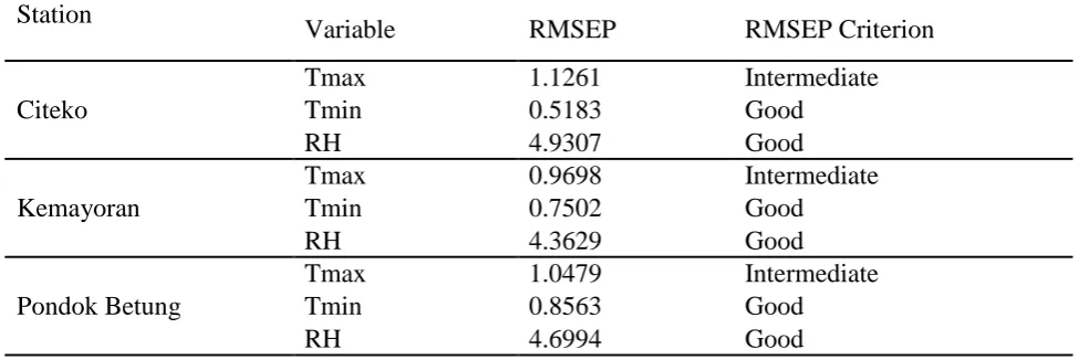
Generally, the RMSEP value of the Tmax modeling using PLS has an intermediate result according to the BMKG criterion. In the other side, the RMSEP value of the Tmin in Citeko, Kemayoran, and Pondok Betung Station has a good result of 1.0857. This PLS modeling is also has a good criterion if used for RH modeling in Citeko, Kemayoran, and Pondok Betung Station, while the RH modeling in Tangerang Station has an intermediate criterion because it holds the RMSEP value of 5.7314. The result of this PLS modeling is then regarded as the MOS model.

Table 13: RMSEP value for PLS in four stations.

Station

Variable RMSEP RMSEP Criterion

Citeko

Tmax 1.1261 Intermediate

Tmin 0.5183 Good

RH 4.9307 Good

Kemayoran

Tmax 0.9698 Intermediate

Tmin 0.7502 Good

RH 4.3629 Good

Pondok Betung

Tmax 1.0479 Intermediate

Tmin 0.8563 Good

12

Tangerang

Tmax 0.9485 Intermediate

Tmin 1.0857 Intermediate

RH 5.7314 Intermediate

3.4 Comparison of Accuracy between NWP Prediction Result and MOS Model Result

The NWP model produces a biased forecast so that it needs a post-processing using the MOS method, i.e. PLS. The percentage of the amount of biased NWP data that can be corrected by the MOS model is shown by the

Percentage Improval (%IM), where the

RMSEPNWP is obtained based on the

comparison of the NWP data on the fifth grid (the nearest grid from the observation station) and the observation data for the Tmax, Tmin, and RH variables. The amount of biased data that can be corrected by the MOS model with the PLS in the four stations are shown in Table 14.

Table 14: The value of RMSEPNWP, RMSEPMOS, dan %IM.

Station Variable RMSEPMOS RMSEPNWP %IM

Citeko

Tmax 1.1261 4.1572 72.9121

Tmin 0.5183 5.1505 89.9369

RH 4.9307 13.0509 62.2195

Kemayoran

Tmax 0.9698 2.9491 67.1154

Tmin 0.7502 1.9110 60.7431

RH 4.3629 7.1804 39.2388

Pondok Betung

Tmax 1.0479 3.3227 68.4624

Tmin 0.8563 1.0812 20.8010

RH 4.6994 7.5821 38.0198

Tangerang

Tmax 0.9485 3.1089 69.4908

Tmin 1.0857 1.3400 18.9776

RH 5.7314 6.5589 12.6164

Table 14 shows that the RMSEP that is obtained from the NWP model is greater than the RMSEP from the MOS model, which means that the MOS model is consistently better to be used to predict the Tmax, Tmin, and RH rather than the NWP model. The MOS model is able to correct from 18.9776% to 89.9369% of the biased NWP for forecasting the Tmin. The same table also shows that the RMSEPNWP in the Citeko Station is the

greatest among the other four stations so that Citeko Station has a %IM that holds the greatest bias corrector. This is because the Citeko Station is located in the mountain area that holds a complex vegetation, therefore producing a big amount of bias for the NWP model.

4. CONCLUSION

13

PLS can solve the NWP problem regarding the relation function and dimension reduction.

The modeling result from this study is recommended to be used for BMKG in forecasting the temperature and humidity because this model is capable to produce a smaller bias compared to the NWP model from the BMKG itself. It must be noted that a method comparison should be done in each station to obtain the best method due to a potential spatial effect that may occur.

5. ACKNOWLEDGEMENT

The entire data used in this study were supported by the Meteorology, Climatology

and Geophysics Agency (BMKG) of

Indonesia. The fund for this study is supported by the Ministry of Research, Technology and Higher Education of Indonesia for the grant of the National Strategic Research 2018.

6. REFERENCES

BMKG. (2006). Uji Operasional dan Validasi

Model Output Statistik (MOS). Jakarta: BMKG.

Boulesteix, Anne-Laure, and Strimmer, K. (2006). Partial Least Squares: A Versatile Tool for the Analysis of

High-Dimensional Genomic Data.

Journal of Briefings in Bioinformatics, 8: 32-44.

Clark, M. P., Hay, L. E., and Whitaker, J. S. (2001). Development of operational hydrologic forecasting capabilities.

American Geophysical Union, Fall Meeting.

Glahn, H. R., and Lowry, D. A. (1972). The Use of a Model Output Statistics

(MOS) in Objective Weather

Forecasting. Applied Meteorology,

1203-1211.

Johnson, R. A., and Winchern, D. W. (2007).

Applied Multivariate Statistical Analysis 6th Edition. United States: Pearson Education.

Joliffe, I. T. (1986). Principal Component Analysis (2nd ed.). New York: Springer-Verlag.

Tjasyono, B. (2004). Klimatologi 2nd Edition. Bandung: ITB.

Wardani, I. K. (2010). Manfaat Prediksi Cuaca Jangka -Pendek Berdasarkan Data Ra-diosonde dan Numerical Weather Prediction (NWP) untuk Pertanian Daerah.

Wilks, D. S. (2006). Statistical Methods in the Atmospheric Sciences 2nd Edition. Boston: Elvesier.

Wold, S., Sjostrom, M., and Eriksson, L. (2001). PLS-regression: a basic tool of

chemometrics. Journal of