A Virtual Delay Generator Design and Its Application

(1)

http://www.sciencepublishinggroup.com/j/ns doi: 10.11648/j.ns.20180301.12

A Virtual Delay Generator Design and Its Application

Gozde Tektas

*

, Cuneyt Celiktas

Department of Physics, Faculty of Science, Ege University, Izmir, Turkey

Email address:

*

Corresponding author

To cite this article:

Gozde Tektas, Cuneyt Celiktas. A Virtual Delay Generator Design and Its Application. Nuclear Science. Vol. 3, No. 1, 2018, pp. 9-15. doi: 10.11648/j.ns.20180301.12

Received: February 25, 2018; Accepted: March 13, 2018; Published: April 8, 2018

Abstract:

A virtual delay generator was developed via software by considering the features of a real ‘gate and delay generator’. The signals supplied from a pulse generator were processed with a preamplifier, an amplifier and a timing single channel analyzer (SCA) and, the SCA output signals were transferred to the real ‘gate and delay generator’ (real instrument) and the virtual delay generator (virtual instrument; VI) simultaneously. They were compared with each other by changing amplitude, delay time and width values of the output signals from both instruments. It was found that the results from the virtual generator were highly in compatible with those of the real one. Obtained results showed that the developed virtual delay generator could be used as the real one.

Keywords:

Virtual Instrument, Virtual Delay Generator, Gate and Delay Generator

1. Introduction

Virtual instrumentation is an interdisciplinary field that merges hardware and software technologies in order to create flexible instruments for control and monitoring applications [1]. Contrary to the real instrument, virtual instrument (VI) is developed in a computer environment through the software. Therefore, it has a lot of advantages according to the real one. One of the most important features is that the virtual instrument is easily designed according to purpose the user’s application.

LabVIEW (Laboratory Virtual Instrument Engineering Workbench) is a graphical programming environment which has become prevalent throughout research labs, academia and industry [2]. LabVIEW can command plug-in data acquisition (DAQ) devices to acquire or generate analog and digital signals. It also facilitates data transfer over General Purpose Interface Bus (GPIB) or Universal Serial Bus (USB), Ethernet or serial port [3]. Various codes can be developed using the functions in LabVIEW library for processing and analyzing of the signals. LabVIEW consists of front panel and block diagram. Codes are developed in block diagram. Front panel is the interface between the user and the VI. Like the user interface of a real instrument, this panel is used to display control buttons and indicators [4].

A digitizer or a data acquisition device is necessary for

processing and analyzing of analog signals supplied from a real instrument such as a radiation detector or a signal generator via software in the computer environment. Analog signals are converted into the digital signals via this device.

A pulse generator is an instrument that generates signals with different amplitudes and frequencies. A preamplifier is used to amplify the signals. An amplifier amplifies the signals from the preamplifier and shapes the signals [5]. A timing single channel analyzer (SCA) is an electronic device with a lower level and a window width variable over the pulse height range. If the input signal is within the window width, it supplies an output logic signal with positive polarity. A ‘gate and delay generator’ accepts the logic pulses in negative or positive polarity, and provides an adjusted delay for each input pulse, and generates output pulses in adjusted amplitudes and widths [6]. An oscilloscope is used to display the signals and to obtain their time and amplitude values. Amplitude is the height of a pulse as measured from its maximum value to its baseline. Signal width is full width of the signal usually taken at its half-maximum [5]. Delay time is the delay value of the signal with regard to time.

(2)

10 Gozde Tektas and Cuneyt Celiktas: A Virtual Delay Generator Design and Its Application

coincidence for 60Co [9], to study of the decay scheme of

244

Cm by an alpha and X-ray coincidence experiment [10]. In the present study, a virtual delay generator was developed since a virtual delay generator has not encountered through the literature browse. In addition, amplitude, delay and width quantities of the output signals from the virtual delay generator were compared with those of the real one.

2. Material and Methods

In this study, a virtual delay generator (virtual instrument;

VI) was developed by considering the features of the Ortec 416A ‘gate and delay generator’ (real instrument). Like a real instrument, delay time, amplitude and signal width values of the output signals can be changed via the knobs in the user interface (Figure 1) of the virtual instrument. “Signal Polarity” button in the interface was used to change polarity of the output signals. Amplitude and signal width values can be set within the range of 2-10 V and 400 ns - 4 µs. Delay time can also be set in the ranges of 0.1-1.1 µs, 1-11 µs and 10-110 µs.

Figure 1. User interface of the VI.

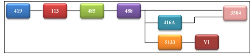
A pulse generator (Ortec 419), a preamplifier (Ortec 113), an amplifier (Ortec 485), a timing SCA (Ortec 488), a ‘gate and delay generator’ (Ortec 416A), an oscilloscope (Gw-Instek 3504), a digitizer (NI-USB 5133), a GPIB (General Purpose Interface Bus) cable and the developed virtual instrument (VI) were used here. Circuit scheme of the measurement system is shown in Figure 2.

As seen in Figure 2, the signals from the generator were sent to the preamplifier. Its output was connected to the amplifier’s input. The amplifier output signals were sent to the timing SCA to generate logic output signals. SCA output was sent to the oscilloscope, the digitizer and the ‘gate and delay generator’, respectively. The ‘gate and delay generator’ output was also sent to the oscilloscope to inspect the signals.

Figure 2. Circuit scheme for the experiment.

It has a sample rate of 4 GS/s [11] and was used to display and to determine the measurement quantities of the ‘gate and delay generator’ output signals.

Data were transferred to the VI by using driver function (NI-SCOPE) of the used digitizer. The logic output signals were supplied via “Pulse Pattern.vi” function. Amplitude, width and delay time of the signals were controlled through this function. Amplitude and width values of the output

(3)

Figure 3. Indication of the cursors.

The digitizer has a sample rate of 100 MS/s and a resolution of 8 bits [12]. It was used to acquire the signals from the timing SCA. The GPIB cable was used to control the oscilloscope through the developed code. Measurements were acquired by stopping the virtual instrument and the oscilloscope simultaneously. Since the pulse generator supplies the signals of 50 Hz, this frequency was kept constant during the measurements. Since the timing SCA supplies only logic output signals with positive polarity, the input signals in positive polarity were examined by the real and virtual instruments. The output signals in positive and negative polarities from the real and the virtual generators (VI) were also inspected as can be seen in the figures below.

When the amplitude and the width values were kept constant to 2 V and 4 µs, the delay time value was adjusted to 10, 60 and 110 µs, respectively. Amplitude values were adjusted to 2, 5 and 10 V when the signal width and the delay time values were adjusted to 4 and 40 µs. When the amplitude and the delay time values were adjusted to 2 V and 40 µs, the signal width values were set to 0.4, 2 and 4 µs.

3. Results

Delay time, signal width and amplitude values of the logic output signals from the real and virtual instruments were compared with each other. Obtained results can be seen in Tables 1-6. Besides, the signal shapes displayed on the VI (Virtual Oscilloscope) were also compared with those of the oscilloscope. These comparisons are shown in Figures 4-9.

3.1. Output Signals with Positive Polarity

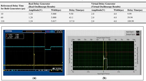
3.1.1. Signals with Different Delay Time

Delay time was adjusted to 10, 60 and 110 µs, respectively. Obtained results are given in Table 1. For 10 µs delay time value, the signal shapes displayed on the VI and the oscilloscope screen are shown in Figure 4.

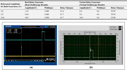
3.1.2. Signals with Different Amplitude

Obtained results for different amplitude values are given in the Table 2. The signals with the amplitude of 10 V are compared in Figure 5.

3.1.3. Signals with Different Width

Signal width was adjusted to 0.4, 2 and 4 µs, respectively. The results are given in Table 3. The signals displayed for the width values of 2 µs are shown in Figure 6.

Table 1. Measurement results for the different delay times.

Referenced Delay Time for Both Generators (µs)

Real Delay Generator (Real Oscilloscope Results)

Virtual Delay Generator (Virtual Oscilloscope Results)

Amplitude(V) Width(µs) Delay Time(µs) Amplitude(V) Width(µs) Delay Time(µs)

10 1.60 4.995 9.50 2.0 4.0 9.99

60 1.60 5.061 63.1 2.0 4.0 59.99

(4)

Figure 4. Signal shapes in (a) the oscilloscope and (b) the VI for 10 µs delay time.

Table 2. Measurement results for the different amplitudes.

Referenced Amplitude for Both Generators (V)

2.0 1.52 5.000 41.6 2.0 4.0 39.99

5.0 5.04 5.000 41.7 5.0 4.0 39.99

10.0 10.8 4.990 41.7 10.0 4.0 39.99

Figure 5. Signal shapes in (a) the oscilloscope and (b) the VI for 10 V.

Table 3. Measurement results for the different signal widths.

Referenced Width for Both Generators (µs)

0.4 1.60 0.395 41.7 2.0 0.4 39.99

2.0 1.52 2.0 41.7 2.0 2.0 39.99

(5)

Figure 6. Signal shapes in (a) the oscilloscope and (b) the VI for 2.0 µs.

3.2. Output Signals with Negative Polarity

3.2.1. Signals with Different Delay Time

Delay time was adjusted to 10, 60 and 110 µs, respectively. Obtained results are given in Table 4. Signal shapes displayed on the VI and the oscilloscope for 10 µs delay time values are shown in Figure 7.

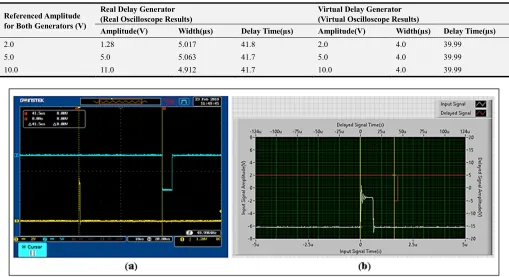
3.2.2. Signals with Different Amplitude

For different amplitude values, obtained results are given

in the Table 5. For 10 V, the signal comparisons are given in Figure 8.

3.2.3. Signals with Different Width

Signal width was adjusted to 0.4, 2 and 4 µs, respectively. Obtained results are given in Table 6. The signals with the width values of 2 µs are compared in Figure 9.

Table 4. Measurement results for the different delay times.

Referenced Delay Time for Both Generators (µs)

10 1.24 5.000 9.50 2.0 4.0 9.99

60 1.28 5.000 63.1 2.0 4.0 59.99

110 1.24 5.017 117.0 2.0 4.0 109.99

(6)

Table 5. Measurement results for the different amplitudes.

Referenced Amplitude for Both Generators (V)

2.0 1.28 5.017 41.8 2.0 4.0 39.99

5.0 5.0 5.063 41.7 5.0 4.0 39.99

10.0 11.0 4.912 41.7 10.0 4.0 39.99

Figure 8. Signal shapes in (a) the oscilloscope and (b) the VI for 10 V.

Table 6. Measurement results for the different signal widths.

Referenced Width for Both Generators (µs)

0.4 2.32 0.401 41.7 2.0 0.4 39.99

2.0 2.24 1.982 41.7 2.0 2.0 39.99

4.0 2.40 5.033 41.7 2.0 4.0 39.99

Figure 9. Signal shapes in (a) the oscilloscope and (b) the VI for 2.0 µs.

4. Discussion

In the present study, a virtual delay generator was developed by considering the features of the real instrument.

(7)

was the same as those of the real one to compare it with the real one. Besides, the output signals with positive or negative polarities could easily be supplied from the VI regardless of the input signal polarity.

Since the delay time between input and output signals could not clearly seen in the values lower than 10 µs due to the oscilloscope and the digitizer capability, delay time was changed from 10 µs to 110 µs.

As can be seen in the Tables, obtained results from the VI were highly in compatible with the adjusted amplitude, signal width and delay time values. Furthermore, they were in good harmony with the results from the real instrument.

When the signal shapes in Figures 4-9, which displayed in the oscilloscope and the VI, were compared, it was shown that they were extremely compatible with each other with respect to the amplitude, width and delay time change. To exact display of the signals on the developed virtual instrument scope as well as the real oscilloscope, sample rate values of the digitizer and the oscilloscope were freely adjusted from each other. So, the signals were displayed in different time scales in the figures.

Delay time values between the input and output signals were determined with the cursors in the oscilloscope. Since the cursors were set by the user, errors might be occurred in reading the data. So, a code was added to the developed VI to remove these type errors.

5. Conclusion

Developed delay generator in the presented study was used instead of a real ‘gate and delay generator’. It was quite successful in generation of the signals like a real one. In addition, it can be used to retard the signals from the order of ns to ms unlike the real one since it was developed in software medium.

Acknowledgements

This work was supported by Scientific Research Foundation of Ege University under project No. 14 FEN 052.

References

[1] Z. Obrenovic, D. Starcevic, E. Jovanov, “Virtual Instrumentation”

https://obren.info/papers/VirtualInstrumentation.pdf. Accessed: 23/02/2018

[2] J. Jerome, “Virtual Instrmentation Using LabVIEW,” PHI Learning Private Limited, 2010.

[3] J. Travis, J. Kring, “LabVIEW For Everyone,” Prentice Hall, 2006.

[4] R. Bitter, T. Mohiuddin, M. Nawrocki, “LabVIEW Advanced Programming Techniques,” CRC Press, 2007.

[5] W. R. Leo, “Techniques for Nuclear and Particle Physics Experiments,” Springer, 1987.

[6]

http://www.ortec-online.com/-/media/ametekortec/manuals/416a-mnl.pdf. Accessed: 23/02/2018

[7]

http://www.ortec-online.com/-/media/ametekortec/third%20edition%20experiments/compto n-scattering.pdf?la=en. Accessed: 23/02/2018

[8]

http://www.ortec-online.com/- /media/ametekortec/third%20edition%20experiments/gamma-gamma-coincidence-angular-correlation.pdf?la=en. Accessed: 23/02/2018 [9] http://www.ortec-online.com/- /media/ametekortec/third%20edition%20experiments/gamma-ray-decay-scheme-angular-correlation-60co.pdf?la=en. Accessed: 23/02/2018 [10] http://www.ortec-online.com/- /media/ametekortec/third%20edition%20experiments/study-

decay-scheme-244cm-alpha-x-ray-coincidence-experiment.pdf?la=en. Accessed: 23/02/2018

[11]

http://www.gwinstek.com/en-global/products/Oscilloscopes/Digital_Storage_Oscilloscopes/ GDS-3000. Accessed: 23/02/2018