Published online April 20, 2014 (http://www.sciencepublishinggroup.com/j/acis) doi: 10.11648/j.acis.20140201.12
A co-design for CAN-based networked control systems
Nguyen Trong Cac, Nguyen Van Khang
School of Electronics and Telecommunications, Hanoi University of Science and Technology, Hanoi, Vietnam
Email address:
[email protected] (N. T. Cac), [email protected] (N. V. Khang)
To cite this article:
Nguyen Trong Cac, Nguyen Van Khang. A Co-Design for CAN-Based Networked Control Systems. Automation, Control and Intelligent Systems. Vol. 2, No. 1, 2014, pp. 6-15. doi: 10.11648/j.acis.20140201.12
Abstract:
The goal of this paper is to consider a co-design approach between the controller of a process control application and the frame scheduling for CAN-Based Networked Control Systems in order to simultaneously improve the Quality of Control (QoC) of the process control and the Quality of Service (QoS) of the CAN-based network. First, we present a way to calculate the closed-loop communication time delay and we compensate this time delay using the pole-placement design method. Second, we propose a hybrid priority scheme for the message scheduling which allows to improve the QoS. Finally, we present a co-design of the communication time delay compensation and the message scheduling, which gives a more efficient Networked Control System.Keywords:
CAN Bus, Networked Control Systems, Message scheduling, Hybrid Priority Schemes, Communication Time Delay, Pole Placement Design, Co-Design1. Introduction
The study and design of Networked Control Systems (NCSs) is a very important research area today because of its multidisciplinary aspect (Automatic Control, Computer Science, and Communication Network). The current objective of NCS design today is to consider a co-design in order to have an efficient control system [1, 2]. Several works [2-6] have considered the co-design problems by combining control and scheduling messages. The works [2, 3] have considered the pole-placement design for time delay compensation and Large Error First (LEF) scheduling algorithm for message scheduling. The value of error is encoded directly into the priority. The higher the error is, the higher the message priority is and vice versa. A limitation is that, we have a wide range of the error value and this is not bounded (for example when the system is unstable, the error is infinite). Mapping these error values in the definite number of priority bits is not an easy task. Paper [4] has considered a hybrid priority scheme for message scheduling using the control signal u. The identifier field of the message which represents the message priority is divided into 2 small fields, the first represents a static priority and the second represents a dynamic priority. However, the limitation of this work is to only use 4 bits for static priority field, so they can determine a maximum number of 16 data flows (or nodes) which is not enough to address all nodes in a NCS. The work [5] only compensates the time delay from the controller to
the actuator, not the closed-loop time delay. The work [6] considers the issue of co-design combines scheduling messages (static priority scheduling) and communication delay compensation.
From the above analysis, we found the same problem co-design of NCS design by combining control system (considering delay compensation issues) and communication networks (considering message scheduling problems) is a new field many investors and should be studied more. Therefore, in this paper will present the co-design of closed-loop time delay compensation and the message scheduling to improve QoC and QoS simultaneously and to have a more efficient NCS.
This paper includes the following sections: the section 2 presents the general context of the study; the section 3 presents the proposal for computation and compensation of closed-loop time delay; the section 4 presents the proposal of a hybrid priority scheme for message scheduling; the section 5 presents the co-design; the conclusion is represented in the section 6.
2. Context of the Study
2.1. Inverted Pendulum Application
Structure diagram of an inverted pendulum mounted on a trolley is shown on Fig. 1.
and the length of l = 0.3m, free fall acceleration g = 9.81m/s2,
θ is the deviation angle of the pendulum, x is the position of the vehicle, u is the force putting into the trolley.
The purpose of the control problem is to move the trolley from position x0 = 0 (initial position) to desired position x1 =
0.1m while keeping the pendulum vertical θ(t) = 0.
Fig 1. Structure diagram of an inverted pendulum mounted on a trolley.
The set point x1 is a position echelon type applied at the
time t=0.5 s. The desired control parameters include: damping coefficient ζ = 0.707, rise time tr = 600 ms, natural
pulsation ωn =1.8tr =3rad/s.
State space model in continuous time [7]:
( ) ( )
( ) ( ) ( )
x Ax t Bu t
y t Cx t Du t
= +
= +
ɺ
(1)
Where:
[
]
0 1 0 0 0
1
0 0 0
,
0 0 0 1 0
( ) 1
0 0 0
1 0 0 0 , 0
mg
M M
A B
M m g
Ml Ml
C D
−
= =
+
−
= =
State-space model in discontinuous time domain with the sampling period h is described as follows [7]:
( ) ( ) ( )
( ) ( ) ( )
x kh h x kh u kh
y kh Cx kh Du kh
+ = Φ + Γ
= +
(2)
Where:
Ah
e
Φ = (3)
0
h As
e dsB
Γ =
∫
(4)The discrete controller is:
( ) d ( )
u kh = −K x kh (5)
The sampling period h is defined by considering the following formula [7]:
0.1≤ωnh≤0.6 (6)
Where ωnis the natural pulsation (rad/s). We choose the
sampling period h = 50 ms.
The state matrix Φ and Γ are calculated by Equation (3) and (4). The state feedback matrix Kd is calculated by using
Ackerman function.
The performances of the discrete time system are as followed: the Overshootof the angle O = 5.07 %, the setting time ts = 0.4 s, and the time responses are shown on Fig. 2.
0 1 2 3 4
-0.04 -0.02 0 0.02 0.04 0.06 0.08 0.1 0.12
Time (s)
x(m),θ(rad)
x
θ
Fig 2. Time responses.
2.2. Implementation of a Process Control Application on a CAN Network
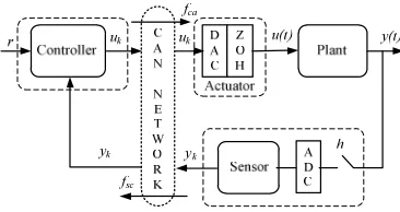
The general model of the implementation of a process control application through a network is shown on Fig. 3.
Fig 3. Implementation of a process control application on a CAN network.
We have three tasks: sensor task, controller task and actuator task. The sensor task is Time-Triggered while the controller task and the actuator tasks are Event-Triggered.
The sensor receives the sampled output yk provided by
the Analog Digital Converter (ADC) and sends a frame including yk to the controller via the communication
network. The controller receives yk from the sensor, then
calculates the control signal uk and sends a frame
including uk to the actuator via the communication
network. The actuator receives uk, converts uk into analog
signal (u(t)) using the Digital Analog Converter (DAC) and then directly applies u(t) to plant. The Zero Order Hold (ZOH) keeps the value u(t) until the reception of the next value.
We have two flows of frames: the Sensor-Controller flow (fsc) concerning the frames going from the sensor to
the controller (denoted “fsc frame”), and the
Controller-Actuator flow (fca) concerning the frames
going from the controller to the actuator (denoted “fca
2.3. Communication Time Delay
Communication time delays in each sampling period consist of 2 components:
• The time delay is due to transferring fsc frames (noted τsc)
which is the duration between the sampling instant (tk, k
= 0, 1, 2…) and the reception instant of this frame by the controller. The time delay τsc includes the waiting time
for medium access and the transmission time of a fsc
frame (noted Dsc)
• The time delay due to transferring fca frames (noted τca)
elapsed from the ready-to-send instant of the fca frame till
the reception instant of this frame by the actuator. The time delay τca includes the waiting time for medium
access and the transmission time of a fca frame (noted
Dca)
Note that Dsc and Dca can be easily calculated based on the
frame length and the network bit rate.
Therefore, the communication time delay of a closed-loop control system is:
sc ca
τ τ= +τ (3)
In this paper, we consider the following hypotheses: • Communication time delay τ < h.
• Computational time in the controller, sensors is neglected.
• There is no data loss.
• Clocks of the sensor and the controller are synchronized,
i.e. the controller recognizes the sampling instant tk.
2.4. Model of NCSs under Communication Time Delay
As shown in Fig. 3, a NCS has a continuous plant (Equation (8)) and a discrete controller (Equation (9)).
( ) ( )
( ) ( ) ( )
x Ax t Bu t
y t Cx t Du t
= + = + ɺ (8)
( ) d ( ), 0,1, 2...
u kh = −K x kh k= (9)
Where x(t) is the state vector, u(t) is the input vector and
y(t) is the output vector, A is the system matrix, B is the input matrix, C is the output matrix, D is the connected matrix. And Kd is the state feedback gain matrix.
State-space model in discrete time domain with the communication time delay τ is described as follows:
0 1
( ) ( ) ( ) ( ) ( ) ( )
( ) ( ) ( )
x kh h x kh u kh u kh h
y kh Cx kh Du kh
τ τ
+ = Φ + Γ + Γ −
= +
(10)
Where Φ, Γ0(τ), Γ1(τ) are the state matrix defined as
follows: 0 0 ( ) h As e dsB τ τ −
Γ =
∫
(4)( )
1
0
( ) A h As
e e dsB
τ τ
τ −
Γ =
∫
(12)State-space model in Equation (10) can be re-written as follows:
1 0
( ) ( ) ( ) ( )
( )
( ) 0 0 ( )
x kh h x kh
u kh
u kh u kh h I
τ τ + Φ Γ Γ = + −
(5)
The discrete controller is:
(
)
(
)
( )
(
)
d
x kh
u kh
K
u kh h
τ
= −
−
(6)Note that the parameters in Equation (10) and Equation (13) depend on h and τ.
2.5. Stability Analysis
Equation (13) can be rewritten as follows:
1 0
( ) ( ) ( ) ( )
( )
( ) 0 0 d ( )
x kh h x kh
K
u kh I u kh h
τ τ τ + Φ Γ Γ = − −
(7)
The matrix of the closed-loop control system is defined as follows:
1
( )
0( )
( )
0
0
cl
K
dI
τ
τ
τ
Φ Γ
Γ
Φ =
−
⋅
(8)With each different sample period, we will find Φcl. We
call k is the number of sampling period; we have the following cases:
2
2 3
3 4
1
1 ( ) (0)
2 ( ) ( ) (0) (0)
3 (2 ) (2 ) (0) (0)
4 (3 ) (3 ) (0) (0)
( ) ( ) (0) (0)
cl
cl cl
cl cl
cl cl
cl
cl cl cl
cl cl
cl cl
k k
cl cl
k x h x
k x h h x h x x
k x h h x h x x
k x h h x h x x
k x kh h x kh −x x
= ⇒ = Φ = ⇒ + = Φ = Φ Φ = Φ = ⇒ + = Φ = Φ Φ = Φ = ⇒ + = Φ = Φ Φ = Φ ⇒ + = Φ = Φ Φ = Φ ⋯
Thus the closed-loop matrix will be the product of the matrix elements, which are calculated as follows:
1 k cl k ∞ =
Φ
∏
(9)Closed-loop matrix in Equation (17) is used to analyze the stability of feedback control systems.
The stability condition is that largest eigenvalue of a closed-loop matrix (Equation (17)) is smaller than 1 [8]:
ax 1
1
k m cl kλ
∞ =
Φ
<
2.6. Global Control System which is Considered
We now present the system which will be analyzed in this work by means of the simulator TrueTime [9], a toolbox based on Matlab/Simulink which allows to simulate real-time distributed control systems.
2.6.1. General Considerations
We implement 8 identical process control applications (noted P1, P2... P8) through a CAN network (Fig. 4). So we
have 24 different nodes connected through a CAN network and 16 data flows (8 fsc and 8 fca flows) sharing the network.
We consider other parameters and conditions as followed: • Bit rate = 125 Kbit/s.
• Data field length of a frame = 8 bytes. Thus, Dsc = Dca =
150 bits [10].
• The sensor tasks are synchronous and have the same sampling period.
Fig 4. Implementation of 8 process control applications on the CAN network.
The scheduling of the frames is done in the MAC layer by means of priorities represented by the Identifier (ID) field of the frame.
Generally, the priorities are static priorities, i.e. each flow has a unique priority (specified a priori out of line) and all the frames of this flow have the same priority. Concerning the priorities, we will consider here either static priorities (i.e. each flow has a unique priority specified out of line) or hybrid priorities (as we said in the introduction) i.e. with two priority levels. One level represents the flow priority which is a static priority. The other level represents the frame transmission urgency. The urgency can be the same for all the frames of the flow and, in this case, the transmission urgency is also a static priority. The urgency can vary (for example, if the conditions of the application, which uses the flow, change) and, in this case, the transmission urgency is a dynamic priority. This concept has a great interest during the transient behavior of systems [12, 13].
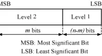
The consideration of hybrid priorities requires structuring the field ID in two levels (Fig. 5) where the Level 1 represents the flow priority and the Level 2 represents the urgency priority [4].
Fig 5. Structure of the ID field.
In the context of the competition based on these hybrid priorities, the frame scheduling is executed by comparing first the bits of the Level 2 (urgency predominance). If the urgencies are identical, the Level 1 (static priorities which have the uniqueness properties) resolves the competition.
2.6.2. Static Priorities Associated to the Fsc and Fca Flows
Here we consider the conclusion shown in [11]: The priority of the fca flow should be higher than the priority of
the fsc flow in order to get the best results. Considering 8
process control applications (P1, P2… P8), each process has
one fsc flow and one fca flow. We call Prio_fca_i and
Prio_fsc_i the priorities of the fsc and fca flows of the process
Pi (i = 1, 2… 8), respectively. The priorities of 16 data flows
are arranged in the following order:
Prio_fca_1 > Prio_fca_2 > … > Prio_fca_8 > Prio_fsc_1 >
Prio_fsc_2 > … > Prio_fsc_8. i.e. the controller has a higher
priority than the sensor and during a sampling period, the order of medium access is arranged as P1, P2, …, P8.
2.6.3. Criteria of the QoC Evaluation
We will consider the time response for the QoC evaluation.
2.6.4. Stability Analysis
As we know the lengths of frames of all processes and the order of medium access, we can calculate the communication time delay of each process. The time delays of P1, P2… P8 are 2.4ms, 4.8ms, 7.2ms, 9.6ms, 12ms, 14.4ms,
16.8ms, 19.2ms respectively. We consider also a time delay of 23.55ms.
The largest eigenvalues of the closed-loop matrix corresponding to the time delay τ above are represented in Table 1. For the case of non-compensation, the higher the delay is, the higher the λmax
( )
Φcl is, which is logical. Forthe 8 processes, the λmax
( )
Φcl <1, thus our system is stable.We see that if the time delay is 23.55ms,
( )
ax 1.009 1
m cl
λ Φ = > , the system will be unstable.
Table 1. Stability Analysis.
ττττ (ms) λmax
( )
Φcl (non-compensation)( )
ax
m cl
λ Φ
(compensation)
2.4 0.000598 0.000597
4.8 0.000623 0.000597
7.2 0.000635 0.000597
9.6 0.000647 0.000597
12 0.000658 0.000597
14.4 0.000669 0.000597 16.8 0.000679 0.000597
19.2 0.0028 0.000597
For the case of Compensation, the λmax
( )
Φcl is equalfor all time delays. It is due to the fact that we have maintained the dominant poles, hence the closed-loop matrix has not been changed, thus the eigenvalues of the closed-loop matrix have not been changed.
3. Proposal for Computation and
Compensation of Time Delays
3.1. Ideas
The goal of this subsection is to propose a way to calculate the closed-loop communication time delay and we compensate this time delay using the pole placement design method in order to improve the QoC for CAN-based NCSs. We consider the implementation of several process control applications on a CAN network. Then we show the interest of the proposed method by comparing the QoC in cases of time delay compensation and of without time delay compensation.
3.2. Computation of Closed-Loop Communication Time Delays
The computation of closed-loop communication time delays is done by the controller in each sampling period.
Concerning the time delay τsc, as the controller has the
knowledge of sampling instants tk (k = 0, 1 …), it can easily
deduce the value of τsc by the time difference between the
reception instant of fsc frames and tk.
Concerning the time delay τca, it cannot be calculated
because the fca frames have not been transmitted yet.
However, due to the hypotheses in section 2.6 (i.e. the priority of the controller is higher than this of the sensor; there is no competition between the controllers; there is no data lost), the controller can immediately send its frame.
Therefore, τca is equal to the duration of a frame
transmission (Dca).
The closed-loop time delay will be computed by the controller as followed:
sc Dca
τ τ= + (11)
3.3. Time Delay Compensation Steps
The compensation for time delays done by the controller in each sampling period has the following steps:
• Step 1: Identifying expected poles including the dominant poles and the other poles [7] which are selected equally to the real part of the dominant pole divided α, with α = 2 ÷ 10.
• Step 2: Computing closed-loop communication time delay.
• Step 3: Computing the controller parameters according to the time delay value in order to maintain the position or the value of the expected poles.
• Step 4: Computing he control signal based on the new control parameters calculated in the previous step.
3.4. Considering the Implementation of the 8 Process Control Applications on CAN Network
We want to show here the interest of the pole-placement design method (which is based on an adaptive controller i.e. the parameters of the controller are modified according to the communication time delay) in comparison with the case where we without time delay compensation (i.e. we have a fixed controller).
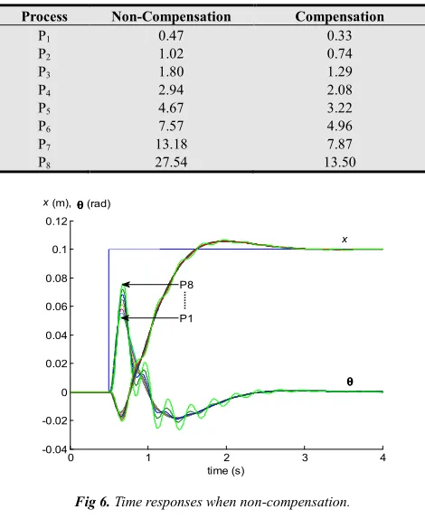
The QoC is represented in Table 2 (∆J/J0 %) and Fig. 6
and Fig. 7.
Table 2. QoC (∆J/J0 %).
Process Non-Compensation Compensation
P1 0.47 0.33
P2 1.02 0.74
P3 1.80 1.29
P4 2.94 2.08
P5 4.67 3.22
P6 7.57 4.96
P7 13.18 7.87
P8 27.54 13.50
0 1 2 3 4
-0.04 -0.02 0 0.02 0.04 0.06 0.08 0.1 0.12
time (s)
x(m),
x
θθθθ
(rad)
θθθθ
P1 P8
Fig 6. Time responses when non-compensation.
0 1 2 3 4
-0.04 -0.02 0 0.02 0.04 0.06 0.08 0.1 0.12
time (s)
x(m),θθθθ(rad)
x
θθθθ
P8
P1
Fig 7. Time responses when compensation.
Remind that the priority of the process Pi is higher than
this of the process Pj. We see in Table 2 for the both cases
In the both Table 2 and Fig. 6 & 7, we can see the improvement of the QoC for the case of compensation compared with the case of non-compensation expressed through smaller values of ∆J/J0 % and less oscillatory time
responses
4. Proposal of a Hybrid Priority Scheme
for Message Scheduling
4.1. Limitations of Static Priorities
Considering static priorities, each node in the network has a unique and fixed priority. Hence, the application which has data flows of low priorities could not get the desired QoS and QoC. For example, we consider a control system with two nodes A and B, in which A has higher priority than B. At the instant t, both A and B have frames to transmit, B has a stronger transmission urgency in order to satisfy the QoS requirement (for example the deadline) but B cannot transmit its frames before the end of the frame transmission of A. That will make the system less efficient.
Other limitations of static priority can be found when we consider time response of process control applications which is characterized by two regimes: transient regime (because of an input change or a noise) and permanent regime (system is in the steady state). In transient regime, frames must be transmitted as soon as possible in order to obtain some QoC requirements such as response time, overshoot, rise time (i.e. frames have high transmission urgencies). Contrariwise, in permanent regime, frames are required to be transmitted quickly (i.e. frames have low transmission urgencies). It is clearly noticed that static priority cannot overcome this problem.
4.2. Hybrid Priorities and Related Works
4.2.1. Idea of Hybrid Priorities
The idea of hybrid priority results from the limitations of static priority presented in the previous section. The idea is that frame priorities can vary depending on transmission urgency. That can be done by restructuring the ID field into 2 small fields as represented in Fig. 5.
Level 2 (m high significant bits) represents transmission urgency which is called dynamic priority part with its value
ID_dyn. The ID_dyn can be changed during system operation and several data flows can share the same ID_dyn. Level 1 (n-m bits) which is called static priority part represents the uniqueness of data flows as its value ID_sta is fixed, unique and specified before system running. The uniqueness means that there are no two or more nodes having the same ID_sta. The term “hybrid priority” means the combination of dynamic priority and static priority.
The idea of this ID field structure was first introduced in [12]. Then other studies [3, 14, 15] also used the similar ID field structure.
The medium access tournament is done firstly by comparing Level 2. If there are several data flows having the
same ID_dyn, Level 1 will determine the only winner allowed to access to the medium.
Remark: With (n-m) ID_sta bits, we can determine 2n-m data flows (or nodes) sharing the network. Therefore, it must be careful when we choose the number of ID_sta bits.
4.2.2. Specifying of the Dynamic Priority
Specifying dynamic priority part requires, firstly, to determine QoC parameter of the process control application which gives information on the transmission urgency, and secondly, to translate these urgencies into dynamic priorities (i.e. computation of dynamic priorities).
Two main QoC parameters using for representing the transmission urgency are steady state error e [3, 14] and control signal u [4, 15]. Some other works use the deadline [12, 13]. With these parameters, the authors proposed different functions for computation of dynamic priorities. The principle is that the higher the values of e, u or deadline are, the higher the dynamic priorities are.
Concerning the works using the error e, they used an extended ID field of 29 bits (16 bits for ID_dyn and 10 bits for ID_sta). The value of e is encoded directly into the ID_dyn value. The first limitation is that, we have a wide range of error value and this is not bounded (for example when the system is unstable, the error is infinite). Mapping these error values in a definite number of priority bits is not an easy task. The second limitation is that, they assume the existence of a master node knowing the current states of all controller nodes. Maintaining a global state in the whole distributed system can be problematic.
The works using the control signal u have overcome the unbounded value by a saturation value us (if u is higher than
us, the dynamic priority is maximum). They used a standard
ID filed of 11 bits (7 bits for ID_dyn and 4 bits for ID_sta). So, they can determine a maximum number of 16 data flows (or nodes) which is not enough to address all nodes in a NCS.
4.3. Proposal
4.3.1. Distributed Aspect
The NCS is totally distributed, i.e. there is not any master node.
4.3.2. ID Field
We use an extended ID field of 29 bits with 11 bits for dynamic priority part, and 11 bits for static priority part. That overcomes the limitation concerning number of ID_sta
bits.
4.3.3. Control Parameters
Both the error e and the control signal u are used for making the dynamic priority.
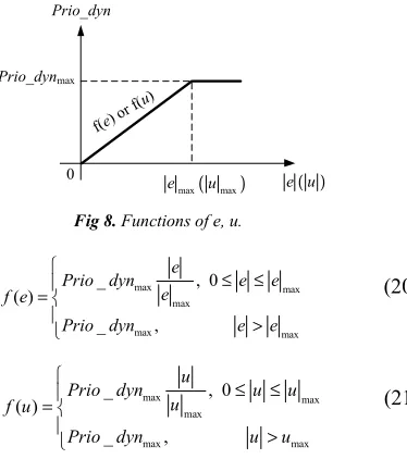
4.3.4. Computation of Dynamic Priorities
The dynamic priority (noted Prio_dyn) is calculated by the controller using functions represented in Fig. 8 and equations (20) & (21). Here, we consider that es and us are
consider the initial continuous control system without the network.
Prio_dyn
0
f(e) o r f(u)
Prio_dynmax
( )
max max
e u e u( )
Fig 8. Functions of e, u.
max max
max
max max
_ , 0
( )
_ ,
e
Prio dyn e e
e f e
Prio dyn e e
≤ ≤
=
>
(20)
max max
max
max max
_ , 0
( )
_ ,
u
Prio dyn u u
u f u
Prio dyn u u
≤ ≤
=
>
(21)
4.3.5. Encoding Priority into ID Field
The dynamic priority part consists of 11 bits which is able to represent 211 = 2048 priority levels from 0 to 2047. The minimum dynamic priority is Prio_dynmin = 0 corresponding
to the ID_dyn of 11 recessive bits (bit 1).
The maximum dynamic priority is Prio_dynmax = 2047
corresponding to the ID_dyn field of 11 dominant bits (bit 0). The relation between the ID_dyn and the Prio_dyn is as follows:
_ 2047 _
ID dyn= −Prio dyn (12)
4.3.6. Implementation of the Hybrid Priority Scheme
Before we present how the hybrid priority scheme works, we should consider the implementation of a process control application on the CAN network as represented on Fig. 9.
We can see how the hybrid priority works. Firstly, concerning the static priority part, this priority of each node is specified before the system running. The subsection 2.6 shows that we have to set static priority of the fca flow (noted
Prio_stafca) higher than that of the fsc flow (noted Prio_stafsc)
in order to get the best results. Here we will consider this conclusion. Secondly, concerning dynamic priority part, its implementation is as follows:
• At the instant tk, the sensor samples the output (yk) and
gets dynamic priority (Prio_dynk-1) sent from the
controller in the previous period (i.e. period starting at
tk-1). After that, the sensor uses this priority
(Prio dyn_ k−1) to send its frame (containing yk) to the
controller.
Fig 9. Implementations of process control applications on a CAN network.
Table 3. QoS (τ ms).
P1 P2 P3 P4 P5 P6 P7 P8 τmax−τmin
Static priority 2.4 4.8 7.2 9.6 12 14.4 16.8 19.2 16.8 Hybrid priority with e 5.9 7.7 9.2 10.4 13.7 12.3 14.4 10.3 8.5 Hybrid priority with u 9.5 9.9 11.0 10.4 12 10.2 12.6 12.9 3.4
0 1 2 3 4 -0.04
-0.02 0 0.02 0.04 0.06 0.08 0.1 0.12
time (s)
0 1 2 3 4 -0.04
-0.02 0 0.02 0.04 0.06 0.08 0.1 0.12
time (s)
0 1 2 3 4 -0.04
-0.02 0 0.02 0.04 0.06 0.08 0.1 0.12
time (s)
x(m), x(m), x(m),
x x x
P1
P8 P8
P1
P8 P1
θθθθ θθθθ θθθθ
θθθθ(rad) θθθθ(rad) θθθθ(rad)
a) Static priority b) Hybrid priority with e c) Hybrid priority with u
• After receiving the fsc frame sent from the sensor, the
controller computes the control signal uk and the
dynamic priority Prio_dynk (by equations (20) & (21))
and sends its frame on the network. Then, the actuator will get uk and apply it to the controlled plant, while the
sensor will get Prio_dynk to use in the next sampling
period (period starting at tk+1).
Concerning dynamic priority using to send the fca frame
by the controller, there are two ways: the first one is that the controller use the Prio_dynk value which has just been
computed [15]; and the second one is to use the Prio_dynmax
[4]. It is evident that the second way ensures that fca frame
will be sent immediately after the reception of fsc frame
(computational time delays in the controller is negligible). Therefore, comparing to the first way, the second way performs a shorter time delay of the closed loop. In this paper, we consider the second one, i.e. the controller uses the
Prio_dynmax to send its frames.
Noting that, at the instant 0 (t0 = 0), the sensor has no
information about the dynamic priority from the controller. Therefore we consider that the sensor uses, at the first time, the Prio_dynmax.
4.4. Implementation of Process Control Application on CAN Network
4.4.1. Communication Time Delay
These time delays are network delays in the communication between the fsc frame (noted τsc) and the fca
frame (noted τca). During each sampling period, time delay
τsc is the time difference between sampling instant and
reception instant of the fsc frame by the controller; the time
delay τca is the time elapsed from the ready-to-send instant
of the fca frame till the reception instant of this frame by the
actuator. Therefore, communication delay in the sampling period is computed as follows:
sc ca
τ τ= +τ (13)
4.4.2. Criteria of the QoS Evaluation
In order to evaluate the QoS, we calculate first the communication time delay τi of the closed loop control system
in each sampling period starting at ti according to the equation
(23), then we compute the average value of theses time delays during the settling time ts by the following formula:
1
1 n i i
n
τ τ
=
=
∑
(24)Where n is the number of sampling period in the settling time.
The smaller the value
τ
is, the better the QoS is.4.4.3. Criteria of the QoC Evaluation
The QoC is considered through the time responses.
4.4.4. Results
a. Quality of Service
We present on the Table 3 the QoS in term of τ of the 8 processes.
For static priority scheme, the process with higher priority has smaller time delay. We see that P1 has the highest priority so
its delay is the smallest while P8 has the lowest priority so its
delay is the biggest. It is logical.
For the hybrid priority scheme (with e and u), we obtain time delays more balanced than these with static priorities. This is the result of the predominant role of the parts “dynamic priority” compared with the parts “static priority”.
The QoS balance can be observed by the difference between the maximum delay and the minimum delay in each priority scheme in the Table 3. We see that these differences are small with hybrid priorities (8.5 ms with e and 3.4 ms with u) while this value is very big with static priorities (16.8 ms).
b. Quality of Control
The QoC is represented in Fig. 10 (time responses). We see also the balances of QoC with hybrid priorities compared with static priorities. It is logical because balances of QoS induce balances of QoC. The conclusions of QoC for different priority schemes are similar to those of QoS. Precisely, for static priority scheme, the higher the priority is, the better the QoC is. And for hybrid priority schemes, the QoCs are more balanced than that of the static priority scheme.
5. Co-Design of Compensation for
Communication Time Delays and the
Message Scheduling
5.1. Ideas
The idea is to combine the frame scheduling scheme based on the hybrid priority and the method of compensation for communication time delay in order to have a more efficient NCSs. However, concerning the close-loop time delay compensation, in the sampling period k, we cannot consider here that the controller can use the value of the close-loop time delay of the sampling period (k-1) because now, taking into account for the dynamic priority used by the sensor task, the time delay (τsc + τca) changes every period.
Then the controller must make the delay compensation in the sampling period k by knowing the close-loop time delay of this sampling period k. We explain now this implementation.
5.2. Principle of the Implementation of the Co-Design
This principle, relatively to the sampling period starting at
tk, is represented on Fig. 11 where we indicate the content of
the fsc and fca frames and the computations done by the
controller. The process of co-design implementation in each cycle starting at tk as follows:
to send a message containing xk to the controller.
• The controller after receiving the signal from the sensor
xk, will perform the following steps:
• The Computations of dynamic priority Prio_dynk based
on the function f(u) and f(e) (by equations (20) & (21)). • Calculations of close-loop communication time delay τ
and the parameters of the controller according to the communication time delay τ, i.e. implementation of the compensation for close-loop communication time delay. • Calculations of the control signal uk.
• Send messages including control signal uk and dynamic
priority Prio_dynk on the network.
Then the actuator will receive the value uk and apply to
control plant, while the sensor will get Prio_dynk to use for
the next period (period starting at tk+1).
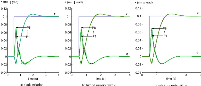
5.3. Performance Evaluation and Summary of Obtained Results
We still consider the implementation of 8 applications (P1,
P2, …, P8) studied in the previous sections.
The time responses are represented on Fig. 12. These results which are represented graphically on obviously show the balanced performances provided by the hybrid priority compared with the static priority and by the co-design compared with the static priority scheme (compensation).
From these results, we can say that, if we have a constraint of performance which cannot be exceeded (not too small), the hybrid priority allows to implement more applications than the static one and, extensionally, the bidirectional relation co-design allows to implement more applications than the static priority scheme (compensation).
Fig 11. Principle of the implementation of the co-design.
0 1 2 3 4
-0.04 -0.02 0 0.02 0.04 0.06 0.08 0.1 0.12
time (s)
0 1 2 3 4
-0.04 -0.02 0 0.02 0.04 0.06 0.08 0.1 0.12
time (s)
0 1 2 3 4
-0.04 -0.02 0 0.02 0.04 0.06 0.08 0.1 0.12
time (s)
x(m),θθθθ(rad) x(m),θθθθ(rad) x(m),θθθθ(rad)
x x x
θθθθ θθθθ θθθθ
P8
P1 P1
P8 P8
P1
a) static priority b) hybrid priority with e c) hybrid priority with u
Fig 12. Time responses when compensation.
6. Conclusion
In this paper, we have presented three following points: • The first is the implementation of the way to calculate
the closed-loop communication time delay and we compensate this time delay using the pole placement design method in order to improve the QoC performances provided by static priorities only.
• The second is the implementation of the hybrid priority
scheme for the message scheduling in order to improve the QoS. The hybrid priority is characterized by, on one hand, a static part representing the uniqueness of the flow, and on the other hand, a dynamic part that represents the urgency of transmission (this dynamic part is expressed from a function of the error and control signal). This hybrid priority gives, in comparison to the static priority case, balanced performances for the different process control applications.
relation QoS and QoC (i.e. co-design) which is the
combination of the between conpensation for
communication time delay and the message scheduling in order to have a more efficient NCSs design. the relation. The results, which are obtained, show the interest of the joint action of the hybrid priorities and the delay compensation (by the hybrid priorities, we introduce the balance aspect compared with the static priority; by the delay compensation, we maintain the balance aspect while improving the QoC and then we can consider the possibility to implement more applications than with the static priority scheme (compensation). The further work should be the following points: the utilization of other compensation methods for time delays (for example, maintenance of the phase margin); the consideration of other types of controller (PID for example) and the consideration of other types of process control applications. Still furthermore, the study of this relation might be also improved by the consideration of theoretical problems (in particulars, stability conditions when the online control law parameters change from sampling period to sampling period).
References
[1] Michael S. Branicky, Vincenzo Liberatore and Stephen M. Phillips, “Networked control system co-simulation for co-design,” American Control Conference, USA, Vol. 4, June 2003, pp. 3341-3346.
[2] Ye-Qiong Song, “Networked Control Systems: From independent designs of the network QoS and the control of the co-design,” 8th IFAC international Conference on Fieldbuses and Networks in Industrial and Embedded Systems, Korea, May 2009, pp. 155-162.
[3] Pau Martí, José Yépez, Manel Velasco, Ricard Villà and Josep M. Fuertes, “Managing Quality-of-Control in network-based control systems by controller and message scheduling co-design,” IEEE Transactions on Industrial Electronics, Vol. 51, No. 6, Dec. 2004, pp. 1159-1167. [4] Xuan Hung Nguyen and Guy Juanole, “Design of Networked
Control Systems on the basis of interplays between Quality of Control and Quality of Service,” 7th IEEE International Symposium on Industrial Embedded Systems, France, June 2012, pp. 85-93.
[5] Y.B. Zhao, G.P. Liu and D. Rees, “Integrated predictive
control and scheduling co-design for networked control systems,” IET Control Theory & Applications, Vol. 2, Issue 1, Jan. 2008, pp. 7-15.
[6] Shi-Lu Dai, Hai Lin, and Shuzhi Sam Ge, “Scheduling and control co-design for a collection of Networked Control Systems with uncertain delays,” IEEE Transactions on control systems technology, Vol. 18, No. 1, Jan. 2010, pp. 66-78.
[7] Karl J. Åström and B. Wittenmark, “Computer controlled systems: theory and design,” 3th Edition, Prentice Hall, 1997. [8] Murat Dogruel and Umit Özgüner, “Stability of a Set of Matrices-A Control heoretic Approach,” 34th Conference on Decision and Control, New Orleans, USA, Vol. 2, Sep. 1995, pp. 1324-1329.
[9] Martin Ohlin, Dan Henrikssonand Anton Cervin, “TrueTime 1.5 - Reference Manual,” Lund Institute of Technology, Sweden, 2007.
[10] Salem Hasnaoui, Oussema Kallel, Ridha Kbaier, Samir Ben Ahmed, “An implementation of a proposed modification of CAN protocol on CAN fieldbus controller component for supporting a dynamic priority policy,” 38th Annual Meeting of the Ind. App., Vol. 1, Oct. 2003, pp. 23-31.
[11] Guy Juanole, Gerard Mouney, Christophe Calmettes, Marek Peca, “Fundamental considerations for implementing control systems on a CAN network,” 6th International Conference on Fielbus Systems and their Applications, Mexico, Nov. 2005, pp. 280-285.
[12] Khawar M. Zuberi end Kang G. Shin, “Scheduling messages on Controller Area Network for real time CIM applications,” IEEE Trans. Robot. Autom, Vol. 13, No. 2, Apr. 1997, pp. 310-314.
[13] Khawar M. Zuberi and Kang G. Shin, “Design and implementation of efficient message scheduling for Controller Area Network,” IEEE Transactions on Computers, Vol. 49, No. 2, Feb. 2000, pp. 182-188.
[14] Manel Velasco, Pau Martí, Rosa Castané, Josep Guardia and Josep M. Fuertes, “A CAN application profile for control optimization in Networked Embedded Systems,” 32nd Annual Conference onIEEE Industrial Electronics, Paris, Nov. 2006, pp. 4638-4643.