Magnetohydrodynamics (MHD) Boundary Layer Flow and
Heat Transfer over Shrinking Sheet with Suction and Stability
Analysis
Nurul Shahirah Mohd Adnan∗1, Norihan Md Arifin2, Norfifah Bachok3, and Fadzilah Md Ali4
1,2,3,4Institute for Mathematical Research, Universiti Putra Malaysia, 43400 UPM
Serdang, Selangor, Malaysia
2,3,4Department of Mathematics, Faculty of Science, Universiti Putra Malaysia, 43400
UPM Serdang, Selangor, Malaysia
∗Corresponding author: iera [email protected]
This case study seeks to examine the fluid flow over shrinking sheet towards suction. This works also investigate the heat transfer in the present of magnetic parameter, heat generation and Lewis number. The basic governing partial differential equations are reduced to a set of ordinary differential equations by using appropriate similarity transformation. To obtain the numerical results, we used MATLAB software. We notice the dual similarity solutions are available in certain range of shrinking sheet parameter. Thus, this results make us continue further in perform the stability analysis by using bvp4c solver in MATLAB software. As expected, our study proved that the solution is stable only the first one and the second solution is not.
Keywords: boundary layer, dual solutions, MHD, stability analysis.
I.
Introduction
The term of boundary layer was introduced by German engineer named Ludwig Prandtl in 1904. According to Prandtl theory, when a flow past an object, the flow region can be divided into two regions. The first region is a thin layer adjoining the solid boundary where the viscous force and rotation cannot be neglected while the second region is an outer region where the viscous force is very small and can be ne-glected. The analysis of boundary layer flow and heat transfer passing stretching/shrinking sheets has gained attention of many researchers in a few years ago due to the importance in engineering applications. (Sakiadis, 1961) was the first researcher that studied the problem of boundary layer flow on a surface of continuous. Then, (Crane, 1970) obtained an exact solu-tion of the boundary layer flow of the Newto-nian fluid caused by the stretching of an elastic
sheet moving in its own plane linearly. Very re-cently, (Zaimi and Ishak, 2015) investigated the problem of boundary layer flow with convec-tive boundary condition and they found that there exist dual solutions for both stretching and shrinking parameter.
(Hamid and Nazar, 2016), (Najib et al., 2017) and (Salleh et al., 2018). The aim of the current paper is to investigate numerically the problem of MHD boundary layer flow and heat transfer towards shrinking with stability analysis.
II.
Mathematical Formulation
Let us consider an incompressible and two di-mensional laminar boundary layer flow over a permeable shrinking sheet. The boundary layer approximations is employed and the equations of the governing problem are as follows:
∂u
∂x +
∂v
∂y = 0 (1)
u∂u ∂x+v
∂u ∂y =ν
∂2u ∂y2 −
σβ02
ρ u (2)
u∂T ∂x +v
∂T
∂y =
κ ρCp
∂2T ∂y2 +
Q ρCp
(T−T∞) (3)
u∂C ∂x +v
∂C ∂y =DB
∂2C
∂y2 (4)
where u and v are velocity component of the fluid along thexand ydirections, respectively.
ν = µ/ρ is the kinematic viscosity where µ is the fluid viscosity and ρ is the fluid density.
σ is the electrical conductivity while β0 is the constant applied magnetic field. T represents temperature and C is the cocentration. Fur-ther, κ refer to thermal conductivity, Cp refer to specific heat of the fluid, Q refer to volu-metric rate of heat generation and DB refer to Brownian diffusion coefficient. And the appro-priate boundary conditions are given by
u=Uw(x) =cx, v=vw,
T =Tw, C=Cw at y= 0
u→0, T −→T∞,
C −→C∞ at y−→ ∞ (5)
Here, c denotes the stretching/shrinking rate where c >0 refers stretching plate whilec <0 refer to shrinking plate. Mass tranfer velocity,
v=vw wherevw <0 refers injection andvw > 0 refer suction and we assumedvw as below:
vw=− √
aνS (6)
Now, we introduced stream function which are defined as u =∂ψ/∂y and v = −∂ψ/∂x. The continuity equation (1) is satisfied by stream function. Then, we assume the similarity trans-formations that defined as follow:
η=yc ν
1/2
, ψ=√aνxf(η),
T =T∞+ (Tw−T∞)θ(η),
C=C∞+ (Cw−C∞)φ(η) (7)
Using equation (7), equations (2), (3) and (4) transformed into nonlinear ordinary differential equations as below:
f000+f f00−f02−M f0 (8)
θ00+P r f θ0+ ∆θ= 0 (9)
φ00+Lef φ0 = 0 (10)
where prime indicates differentiation with re-spect to η. M = σβ20
aρ refer to the magnetic parameter and P r = µCp
κ denotes the Prandtl number. Then, ∆ = ρaCQ
p is the heat source
(∆<0) or sink (∆>0) parameter whileLe= ν
DB is Lewis number. The transformed
bound-ary conditions are:
f(0) =S, f0(0) =λ, θ(0) = 1, φ(0) = 1
and f0(∞)→0, θ(∞)→0, φ(∞)→0 (11)
III.
Stability Analysis
In order to perform stability analysis, we need to consider the unsteady problem. Equation (1) holds, while equations (2)-(4) are replaced by
∂u ∂t +u
∂u ∂x+v
∂u ∂y =ν
∂2u ∂y2 −
σβ02
ρ u (12)
∂T ∂t +u
∂T ∂x+v
∂T
∂y =
κ ρCp
∂2T ∂y2 +
Q ρCp
(T−T∞)
(13)
∂C ∂t +u
∂C ∂x +v
∂C ∂y =DB
∂2C
∂y2 (14)
wheretdenotes the time. Then, based on simi-larity transformations in (7), we introduced the new dimensionless variables as follow:
η=y c
ν 1/2
, ψ=√aνxf(η, τ),
T =T∞+ (Tw−T∞)θ(η, τ),
C=C∞+ (Cw−C∞)φ(η, τ), τ =ct (15)
Thus, equations (2)-(4) changed to the follow-ing equations:
∂3f
∂η3 +f
∂2f
∂η2 −
∂f ∂η 2 −M ∂f ∂η − ∂ 2f
∂η∂τ = 0
(16)
∂2θ ∂η +P r
f∂θ ∂η +λθ− ∂θ ∂τ
= 0 (17)
∂2φ
∂η2 +Le
f∂φ ∂η − ∂φ ∂τ
= 0 (18)
alongside boundary conditions as follows:
f(0, τ) =S, ∂f
∂η(0, τ) =λ, θ(0, τ) = 1, φ(0, τ) = 1
∂f
∂η (∞, τ)→0, θ(∞, τ)→0, φ(∞, τ)→0
(19)
To test the stability of the solution f(η) =
f0(η), θ(η) = θ0(η) and φ(η) = φ0(η) satis-fying the boundary value problem (8)-(11), we write:
f(η, τ) =f0(η) +e−γτF(η, τ),
θ(η, τ) =θ0(η) +e−γτH(η, τ), (20)
φ(η, τ) =φ0(η) +e−γτG(η, τ),
whereγis an unknown eigenvalue. F(η),H(η) andG(η) are small relative tof0(η),θ0(η) and
φ0(η). Next, differentiate equation (20) and the substitute into equations (16)-(18) to ob-tain eigenvalue problem as below:
F0000+f0F000+f000F0−2f00F00−M F00+γF00 = 0, (21)
H000+P r f0H00 +θ 0
0F0+ ∆H0+γH0
= 0,
(22)
G000+Le f0G00+φ 0
0F0+γG0
= 0 (23)
together with the new boundary conditions
F0(0) = 0, F00(0) = 0, H0(0) = 0, G0(0) = 0,
F00(η)→0, H0(η)→0, G0(η)→0 (24)
To be noted, the stability of the problem can be determine by the smallest eigenvalueγ. There-fore, the condition F00(η) → 0 as η → ∞ has been put at rest as suggested by (Harris et al., 2009) and for fixed value of eigenvalue, γ.
IV.
Results and Discussion
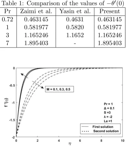
Be-sides, to support the results obtained, we com-pared our results with those reported by (Za-imi et al., 2014) and (Yasin et al., 2016) as il-lustrated in Table 1 by considering the values of ∆ = S = M = Le = 0 and λ = 1. The comparison shows very good agreement. The respective results are given to carry out the in-fluences of several kind of parameters on the parametric study such as magnetic parameter,
M, heat source or sink parameter, ∆ and Lewis number,Le.
Table 1: Comparison of the values of−θ0(0) Pr Zaimi et al. Yasin et al. Present 0.72 0.463145 0.4631 0.463145
1 0.581977 0.5820 0.581977 3 1.165246 1.1652 1.165246
7 1.895403 - 1.895403
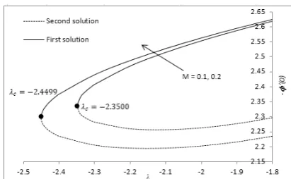
Figure 1: Velocity profile for various values of
M
We now consider velocity profilesf0(η) as illus-trated in Figure 1 for selected values of mag-netic parameter,M when we consider the value of P r = 1, ∆ = 0.1, S = 3, λ = −2 and
Le = 1. From Figure 1, as magnetic pa-rameter, M increase, the momentum bound-ary layer thickness decrease. This is due to the magnetic force acting on the sheet increases as well, causing the boundary layer thickness to become smaller. In addition, Figure 2 shows the various values of heat source/sink param-eter, ∆ on temperature profile θ(η). Increas-ing heat generation (∆ > 0) significantly
ac-Figure 2: Temperature profile for various val-ues of ∆
Figure 3: Concentration profile for various val-ues of Le
celerates the flow and also increases tempera-ture magnitudes. Conversely, with a heat sink (∆ < 0) present, the flow is retarded which means that momentum boundary layer thick-ness is lowered. Then, thermal boundary layer thickness is reduced. Next, as shown in Figure 3, when Lewis number,Leincrease, the bound-ary layer thickness decrease.
Figure 4: Velocity profile for various values of
S
Figure 5: Temperature profile for various val-ues of S
Figure 6: Concentration profile for various val-ues of S
On other hand, the thickness of the thermal boundary layer is decreasing when we increase the value of suction parameter, S. Hence,
suction parameter, S with larger value will enhance the heat transfer rate more quickly compared to smaller suction parameter,S.
Figure 7: Skin friction coefficient for various values ofM
Figure 8: Local Nusselt number for various val-ues of M
Figure 9: Concentration gradient for various values ofM
lo-cal Nusselt number and concentration gradient with magnetic parameter, M are show in Fig-ure 7-9. Based on FigFig-ure 7, it is seen that upon increasing of magnetic parameter,M, the skin friction coefficient is increase. In fact, the value of f00(0) is positive when λ < 1. Physically positive value of f00(0) means the fluid exerts a drag force on the solid boundary. Normally, when λ= 1, f00(0) = 0. This is due to the fact that there is no friction at the friction at the fluid-solid interface when the fluid and the solid boundary move with the same velocity. Be-sides, from Figure 8, the local Nusselt number increase when the increasing of the magnetic parameter, M. It is also good to know that an increment of magnetic parameter, M leads to a increase in the ratio of thermal conductivity. Next, Figure 9 also shows that concentration gradient increase as the magnetic parameter,
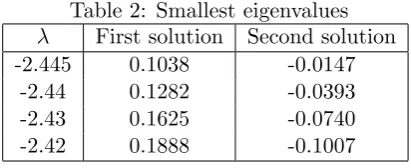
M is increase. These Figures admit dual so-lution when λ > λc while when λ < λc, no similarity solutions exist for equations (8)-(10). From Figure 1-9, it is shown that there exist dual solutions for this current problem. Hence, an analysis of stability is performed in order to identify which solution is most stable between two solutions. The results displayed in Table 2 states that first solution is in positive value while second solution in negative value. Hence, we can finally conclude that the first solution is stable and significantly realizable meanwhile the second solution is in opposite manner.
Table 2: Smallest eigenvalues
λ First solution Second solution -2.445 0.1038 -0.0147
-2.44 0.1282 -0.0393 -2.43 0.1625 -0.0740 -2.42 0.1888 -0.1007
V.
Conclusion
The study of a stability analysis on MHD boundary layer flow and heat transfer towards shrinking sheet with suction has been nu-merically analyzed and discussed in detail in
this paper. It was found that the involv-ing parameters-specifically magnetic parame-ter, heat generation parameparame-ter, suction param-eter and Lewis number significantly affected the flow field. Then, we noticed that there are dual solutions. Hence, we continue further in perform stability analysis to identify which solution is stable. It is found that dual solu-tion exist when λ > λc. The λc = −2.3500 when magnetic parameter,M = 0.1 while when we consider for M = 0.2, the λc = −2.4499. Lastly, we can conclude that the first solution is always in stable state while the second solu-tion is not.
Acknowledgements
We would like to thank Universiti Putra Malaysia for supporting this project under Geran Putra IPS (Project number: GP-IPS/2018/9624700).
References
[1] Lawrence J Crane. Flow past a stretching plate. Zeitschrift f¨ur angewandte Mathe-matik und Physik ZAMP, 21(4):645–647, 1970.
[2] Rohana Abdul Hamid and Roslinda Nazar. Stability analysis of mhd ther-mosolutal marangoni convection bound-ary layer flow. In AIP Conference Pro-ceedings, volume 1750, page 030022. AIP Publishing, 2016.
[3] SD Harris, DB Ingham, and I Pop. Mixed convection boundary-layer flow near the stagnation point on a vertical surface in a porous medium: Brinkman model with slip. Transport in Porous Media, 77(2): 267–285, 2009.
stability analysis. In AIP Conference Proceedings, volume 1974, page 020083. AIP Publishing, 2018.
[5] JH Merkin. On dual solutions occurring in mixed convection in a porous medium. Journal of engineering Mathematics, 20 (2):171–179, 1986.
[6] N Najib, N Bachok, NM Arifin, FM Ali, and I Pop. Stability solutions on stagna-tion point flow in cu-water nanofluid on stretching/shrinking cylinder with chem-ical reaction and slip effect. InJournal of Physics: Conference Series, volume 890, page 012030. IOP Publishing, 2017.
[7] Byron C Sakiadis. Boundary-layer behavior on continuous solid surfaces: I. boundary-layer equations for two-dimensional and axisymmetric flow. AIChE Journal, 7(1):26–28, 1961.
[8] Siti Nur Alwani Salleh, Norfifah Bachok, Norihan Md Arifin, Fadzilah Md Ali, and Ioan Pop. Stability analysis of mixed con-vection flow towards a moving thin needle in nanofluid. Applied Sciences, 8(6):842, 2018.
[9] Rajesh Sharma, Anuar Ishak, and Ioan Pop. Stability analysis of magnetohydro-dynamic stagnation-point flow toward a stretching/shrinking sheet. Computers & Fluids, 102:94–98, 2014.
[10] Mohd Hafizi Mat Yasin, Anuar Ishak, and Ioan Pop. Mhd heat and mass transfer flow over a permeable stretch-ing/shrinking sheet with radiation effect. Journal of Magnetism and Magnetic Ma-terials, 407:235–240, 2016.
[11] K. Zaimi and A. Ishak. Boundary layer flow and heat transfer over a permeable stretching/shrinking sheet with a con-vective boundary condition. Journal of Applied Fluid Mechanics, 8(3):499–505, 2015. ISSN 1735-3572.