A new code transformation technique for nested loops

(1)

A new code transformation technique for nested loops

Ivan ˇSimeˇcek1_{and Pavel Tvrd´ık}1 Department of Computer Systems, Faculty of Information Technology, Czech Technical University in Prague, 160 00,

Prague, Czech Republic {xsimecek,pavel.tvrdik}@fit.cvut.cz

Abstract. For good performance of every computer program, good cache utiliza-tion is crucial. In numerical linear algebra libraries, good cache utilizautiliza-tion is achieved by explicitloop restructuring(mainlyloop blocking), but it requires a complicated memory pattern behavior analysis. In this paper, we describe a new source code transformation calleddynamic loop reversalthat can increase temporal and spatial locality. We also describe a formal method for predicting cache behavior and eval-uate results of the model accuracy by the measurements on a cache monitor. The comparisons of the numbers of measured cache misses and the numbers of cache misses estimated by the model indicate that the model is relatively accurate and can be used in practice.

Keywords:Source code optimization, loop transformations, model of cache behav-ior.

1. Introduction

1.1. General

Due to the increasing difference between memory and processor speed, it becomes critical to minimize communications between main memory and processor. It is done by addition of cache memories on the data path. The memory subsystem of nowadays processors is organized as a hierarchy in which the latency of memory accesses increases rapidly from one level of hierarchy to the next. Numerical codes (e.g. libraries such as BLAS [9] or LAPACK [2]) are now some of the most demanding programs in terms of execution time and memory usage. These numerical codes consist mainly of loops. Programmers and op-timizing compilers often restructure a code to improve its cache utilization. Many source code transformation techniques have been developed and used in the state-of-the-art

op-timizing compilers. In this paper, we consider the following standard techniques:loop

(2)

unrolling,loop blocking,loop fusion, andloop reversal[15, 30, 32, 8]. Models for pre-dicting the number of cache misses have also been developed to have detailed knowledge about the impacts of these transformation techniques on the cache utilization. The existing literature aimed at the maximal cache utilization within numerical codes focused mainly on regular memory accesses, but there is also an important subset of numerical codes where memory accesses are irregular (e.g. for computations with sparse matrices). As far as we know, there is no transformation technique that can improve the cache behavior for regular and irregular codes.

The main result of this paper is a description of a new transformation technique, called

dynamic loop reversal, shortly DLR. This transformation technique can lead to better

cache utilization (even for codes with irregular memory accesses) due to the improved temporal and spatial locality with no need to analyze the memory pattern behavior.

In Section 2, we introduce the basic terminology (the used model of the cache archi-tecture and the basic sparse matrix storage format). In Section 3, we briefly discuss the motivation that lead us to the design of DLR transformation. In order to incorporate the DLR into compilers, we propose models for predicting the number of cache misses for DLR in Section 4. In Section 5, we describe experiment’s settings and configurations used for measurement the effects of DLR. In Section 6, we measure and evaluate the effects of DLR (e.g. performance, cache miss rate) on example codes. In Section 7, we discuss an idea of an automatic compiler support of DLR to optimize nested loops.

1.2. Related works

There are many existing source code transformation techniques (for details see [15, 30, 32]). Models for enumeration of the number of cache misses have also been developed see ([27, 1, 33]) for predicting the impacts of these transformation techniques on the cache utilization. But only few of existing papers also aim at codes with irregular memory ac-cesses (e.g. computations with sparse matrices). In [8], optimizations for multicore stencil (nearest-neighbor) computations are explored. This class of algorithms is used in many PDE solvers. Authors develop a number of effective optimization strategies and propose an auto-tuning environment.

The other approach for optimization of multicore stencil computations is proposed in [21]: programmer should specify a stencil in a domain-specific stencil language [17] — Pochoir language. The resulting optimizations are derived from this specification.

There are also many algorithms and storage formats designed for the acceleration of the sparse matrix-vector multiplication (e.g. [29, 11, 25, 12]).

But all mentioned papers are focused only on the specific operation, the proposed DLR transformation is more general and can be applied to non-specific codes.

2. Terminology

In the paper, we assume that all elements of vectors and matrices are of the typedouble

(3)

h

s·BS BS

Fig. 1.Description of the cache parameters.

2.1. The cache architecture model

We consider a most used model of theset-associative cache data cache (for details see

[14]). The number of sets is denoted ash(see Figure 1). One set consists ofsindependent

blocks. The size of the data cache in bytes is denoted as DCS. The cache block size

in bytes is denoted asBS. Then DCS = s·BS·h. The size of the typedouble is

denoted asSD. We consider onlywrite-backcaches with anleast recently used (LRU)

block replacementstrategy.

We consider two types of cache misses:

– Compulsorymisses (sometimes calledintrinsicorcold) that occur when new data is

loaded into empty cache blocks.

– Thrashingmisses (also called cross-interference, conflict, orcapacity misses) that

occur because the useful data was replaced prematurely from the cache block.

In modern architectures, there are three level of caches, but we can consider each level independently. Some caches are unified (for data and instructions), but we assume them as data caches because the size of (most frequent) code is negligible.

2.2. Compressed sparse row (CSR) format

A matrixAof ordernis considered to besparseif it contains much less nonzero elements

thann2_{otherwise it is considered as}_dense_{. Some alternative definitions of sparse matrix}

can be found in [22]. The most common format (see [10, 11, 23, 25]) for storing sparse

matrices is thecompressed sparse row(CSR) format. The number of nonzero elements is

denoted asNZA. A matrixAstored in the CSR format is represented by three linear arrays

ElemA,AddrA, andCiA(see Figure 2 b). ArrayElemA[1, . . . ,NZA]stores the nonzero

elements ofA. ArrayAddrA[1, . . . , n+ 1]contains indexes of initial nonzero elements of

rows ofA. Hence, the first nonzero element of rowjis stored at indexAddrA[j]in array

ElemA, obviouslyAddrA[1] = 1andAddrA[n+ 1] =NZA. ArrayCiA[1, . . . ,NZA]

contains column indexes of nonzero elements ofA. The density of a matrixA(denoted

asdensity(A)) is the ratio betweenNZAandn2.

3. Code restructuring

In this section, we propose a new optimization technique calleddynamic loop reversal(or

(4)

1 2 3 4 5 6 7 8 9 1

2 3 4

a)

arrayAddrA arrayCiA

arrayElemA

1 2 4 6 2 3 4 2 3 5 6 7 3 4 0 4 7 12 14

b)

Fig. 2.a) Example of a sparse matrix, b) Representation of this matrix in the CSR format.

3.1. Standard static loop reversal

In standard loop reversal, the direction of the passage through the interval of a loop iter-ation variable is reversed. This rearrangement changes the sequence of memory require-ments and reverses data dependencies. Therefore, it allows further loop optimizations (e.g. loop unrolling or loop blocking) in general.

Example code 1 1: fori←n,2do

2: B[i]←B[i] +B[i−1];

3: fori←2, ndo 4: A[i]←A[i] +B[i];

Example code 1 represents a typical combination of data-dependent loops whose data dependency can be recognized automatically by common compiler optimization

tech-niques. However, both loops arereversible(it means that it is possible to alternate the

sense of the passage). The reversal of the second loop and loop fusion can be applied and the reuse distances (for the definition of the reuse distance see Section 4.1) for the

memory transactions on arrayBare decreased.

Example code 2Loop reversal and loop fusion applied to Example code 1

1: fori←n,2do

2: B[i]←B[i] +B[i−1];

3: A[i]←A[i] +B[i];

(5)

Example code 3

1: fori←1, ndo .Loop 1

2: s←s+A[i]∗A[i];

3: norm←√s;

5: A[i]←A[i]/norm;

However, the application of the loop reversal to the second loop decreases the reuse distances.

Example code 4Loop reversal applied to Example code 3

2: s←s+A[i]∗A[i];

3: norm←√s;

4: fori←n,1do .Loop 2

5: A[i]←A[i]/norm;

The problem is that in this case (and in other similar cases), the compiler heuristics for the decision which loop to reverse to minimize reuse distances is complicated. This idea was used in [23] for the acceleration of Conjugate Gradient method.

A

_array

array

=1

i

₌₁

Iteration

n

i

n

R

euse di

st

anc

e

(Loop 2)

(

Loop 1

)

first access

reused

not reused

(6)

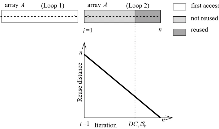
3.2. Effect of the static loop reversal on cache behavior

If the size of arrayAis less than the cache size (nSD≤DCS), then Example code 3 and

4 are equivalent as to the cache utilization. However, if the size of arrayAexceeds the

cache size, then no elements ofAare reused in Example code 3, whereas the lastk=BS

SD

elements ofAare reused within the second reversed loop. Thus, loop reversal improves

the temporal locality (see Figures 3 and 4 for the comparison of reuse distances).

A A

array array

=1 =1

Iteration

not reused

reused first access

i

(Loop 1) (Loop 2)

n

R

euse di

st

anc

e

/SD S

DC

n i

Fig. 4.Reuse distances inExample code 4(Example code 3after loop reversal).

3.3. Dynamic loop reversal

The static loop reversal is used to reverse data-dependency in one dimension. This moti-vated us to generalize this idea, and therefore we designed another optimization for nested reversible loops based on loop reversal. Consider the following code (Example code 5):

Example code 5 1: fori←1, ndo 2: s←0;

3: forj←1, ndo

4: s←s+A[i][j]∗x[j];

(7)

loop reversal in every iteration of the outer loop. This is why we call it adynamic loop

reversal, orDLRfor short. Example code 5 is a candidate for such a transformation.

Example code 6DLR applied to Example code 5

1: fori←1, ndo 2: s←0;

3: ifiis oddthen 4: forj←1, ndo

5: s←s+A[i][j]∗x[j];

6: else

7: forj←n,1do

8: s←s+A[i][j]∗x[j];

This transformation will be denoted as DLR(i→j). For large arrays, this

transforma-tion (the result is Example code 6) leads to even better temporal locality than the original Example code 5, because it reduces the reuse distances, and some data resides in the cache from the previous iteration. On the other hand, the saving of the number of cache

misses in one iteration of the outer loop is bounded byDCS/BS. Therefore,DLRhas a

significant effect if the cache size is comparable to the sum of the affected array sizes in

one iteration of the outer loop. The necessary condition for applyingDLRis that the inner

loop must be reversible.

Possible implementations of DLR The straightforward implementation, described above by the code “DLR applied to Example code 5”(Example code 6), leads to an overhead due to one additional conditional jump that is hard to predict due to its pattern. We call it “im-plementation variant A”.

We propose the other possible implementation as follows.

Example code 7DLR applied to Example code 5

1: fori←1, nstep2do 2: s←0;

3: forj←1, ndo

4: s←s+A[i][j]∗x[j];

5: forj←n,1do

6: s←s+A[i+ 1][j]∗x[j];

7: ifnis oddthen 8: forj←1, ndo

9: s←s+A[n][j]∗x[j];

The second implementation (Example code 7) leads to a faster code, since the

condi-tional jump inside thei-loop is eliminated, but in fact, it is based on the loop unrolling.

(8)

Possible interference of DLR with heuristics in optimizing compilers On the other hand, DLR may have a disadvantage due to the fact that it can confuse optimizing com-pilers and hinder further loop optimizations. For example, in Example code 5, there are two nested loops and after the application of DLR (implementation variant A), the code contains also a conditional branch that is non-trivial for the compiler heuristics (see [33]).

The application of DLR on triple-nested loops In the previous text, DLR was applied to double-nested loops, but it can also be applied to triple-nested loops. Consider the following code skeleton (Example code 8):

Example code 8 1: fori←1, ndo 2: forj←1, ndo 3: fork←1, ndo 4: (* loop body *)

In Example code 8, there are three options how the DLR can be applied:

– on thei-loop: DLR(i→j),

– on thej-loop: DLR(j→k),

– both transformations: DLR(i→j) and DLR(j→k).

The last option lies in the composition of two transformations DLR(i→j) and DLR(j→

k). This composition we will denoted as DLR(i→j→k). In this case, the effect of DLR

is twofold: DLR(i→j) (on the outer pair of the loops) can improve a temporal locality

inside the L2 cache and DLR(j → k) (on the inner pair of the loops) can improve a

temporal locality inside the L1 cache.

3.4. Comparison and possible combinations of DLR and other loop restructuring techniques

Loop unrolling Loop unrolling has two main effects. Firstly, it makes the sequential code longer, so it may improve the data throughput, because the instructions could be bet-ter scheduled and the inbet-ternal pipeline could be betbet-ter utilized. Secondly, the number of test condition evaluations drops according to the unrolling factor. In general, the loop un-rolling concentrates on maximizing the machine throughput, not on improving the cache behavior.

(9)

Loop tiling (blocking) Loop tiling (sometimes called loop blocking or iteration space tiling) is one of the advanced loop restructuring techniques (for details see [7, 31, 5, 6, 20, 28]). The compiler can use it to increase the cache hit rate. The following code (Example code 9) is an example of an application of the loop tiling technique.

Example code 9

1: fori1←1, nstepBf do 2: forj1←1, nstepBfdo 3: fork1←1, nstepBf do

4: fori←i1,min(i1+Bf−1, n)do 5: forj←j1,min(j1+Bf−1, n)do 6: fork←k1,min(k1+Bf−1, n)do 7: C[i][j]←C[i][j] +A[i][k]∗B[k][j];

One possible motivation for using this technique is the fact that theloop range(i.e.,

the size of the array traversed repeatedly within the loop) is too big and exceeds the data

cache sizeDCS. Thus, the loop should be split into two loops: the outer loop (out-cache

loop) and the inner loop (in-cache loop). The valueBf is called atiling or block factor,

whose its optimal value depends on the cache size.

The loop tiling and DLR can be easily combined. DLR can be applied on every pair

of immediately nested loop, but it is useless to apply it for in-cache loops (i-loop, j

-loop, andk-loop). We consider loop tiling a competitor to DLR and thus we performed

experiments with both. These quantitative measurements of the effects of these techniques are presented in Section 6.4.

4. Analytical model of the cache behavior for DLR

To estimate parameters for loop restructuring techniques, modern compilers use the

poly-tope model[32, 33]. We will present three cache behavior models based on reuse distances

(shortly RD) that can be derived from the polytope model.

4.1. Cache miss model with reuse distances

This model is inspired by the model introduced in [4, 3, 24]. We will call it basic RD

model.

Definition 1. Consider an execution of an algorithm on the computer with load/store architecture and assume that the addresses of memory transactions form a sequence

P[1, . . . , n] = [addr1, . . . , addrn]. ThenP is called asequence of memory access ad-dressesandP[i] =addriis thei-th transaction with memory addressaddri. Thereuse distanceRD(t), wheret∈(1, n], is the number ofdifferentmemory addresses accessed

between two uses of the addressP[t]. Formally, ifP[t] =addrtand(t)>0is the

mini-mal integer number such thatP[t−(t)] =addrt, thenRD(t) =|{P[t−(t)], . . . , P[t−

(10)

Obviously, in the above definition,RD(t)≤(t)orRD(t) =∞. The notion of reuse distances can be used for developing a simple cache miss model based on estimating the

numbers of thrashing misses in fully-associative (h= 1) caches. IfRD(t)> DCS/SD,

then the content of the cache block from the memory addressP(t)is replaced by a new

value and a cache miss occurs. IfRD(t) = ∞, then a compulsory miss occurs,

other-wise a thrashing miss occurs. Remember that we assume only caches with LRU block replacement strategy.

In this basic RD model, the spatial locality of the cache memory is not considered, i.e.,

it is assumed that a cache block contains exactly one array element (BS=SD). However,

BS = c·SD, wherec is typically 4 or 8 in modern processors, and therefore, spatial

locality must be taken into account in order to create a more realistic model.

4.2. The cache miss model with generalized reuse distances

To address this drawback of the basic RD model, we define a more general form of reuse

distances. We call this modelgeneralized RD model.

Definition 2. Consider a sequence of memory access addressesP[1, . . . , n]. Address

addri fromP is mapped onto a cache block marked by tagtagi computed by the

cor-responding cache memory mapping function. Then P0[1, . . . , n] = [tag1, . . . , tagn] is

called asequence of cache memory tags. Then thegeneralized reuse distanceGRD(t),

wheret∈(1, n], is defined as the number ofdifferentcache blocks accessed between two

uses of the tagP0[t]. Formally, ifP0[t] =tagtand(t)>0is the minimal integer number

such thatP0[t−(t)] = tagt, thenGRD(t) = |P0[t−(t)], . . . , P0[t−1]|. If such an

(t)does not exist, thenGRD(t) =∞.

The generalized reuse distances can be useful for estimating the numbers of cache

misses. IfGRD(t)> DCS/BS, then the content of cache blockP0(t)is replaced by a

new value, and a cache miss occurs (ifGRD(t) = ∞, then a compulsory miss occurs;

otherwise, a thrashing miss occurs).

Both cache miss models based on the reuse distances (RD and GRD) has several drawbacks:

– Reuse distances for a given memory address or cache memory tag vary in time.

Intervals of reuses are not the same during the execution (RD(t1) 6= RD(t2)for

P[t1] =P[t2]).

– The mapping function of the cache memory is not considered. Essentially, the cache

is assumed fully-associative (h= 1).

4.3. Simplified cache miss model for DLR

Even the basic RD model is too complicated for modeling the cache behavior of DLR in real applications. Hence, we introduce the other model that is even more simplified.

The model will be calledsimplified RD model. We use this model for the enumeration

of cache misses saved by DLR. To derive an analytical model of a DLR effect on the cache behavior, consider the following code skeleton (Example code 10) representing

most frequent memory access patterns during a matrix computation (k, l are the small

(11)

Example code 10 1: statement1; 2: fori←i1, i2do 3: statement2; 4: forj←j1, j2do 5: statement3;

6: · · · ←B[k∗j+l]; .Memory operation of typeα 7: · · · ←B[k∗i+l]; .Memory operation of typeβ 8: · · · ←A[i][k∗j+l]; .Memory operation of typeγ 9: · · · ←A[j][k∗i+l]; .Memory operation of typeδ 10: statement4;

11: statement5;

We consider the following simplifying conditions:

A1 We assume that all matrices are stored in the row-major order.

A2 We assume thatstatements1−5contain only local computation with register operands.

That is, we assume thatstatements1−5have zero cache effects and the only memory

accesses are memory operations of typeα−δ.

A3 We assume that the generalized reuse distances depend on the exact ordering of

mem-ory operations (inside thej-loop) only slightly and so does the number of cache

misses.

A4 We do not distinguish between load and store operations.

A5 We assume that the cache memory is big enough to hold all the data for one iteration

of the (inner)j-loop.

A6 We assume that the cache memory is not able to hold all the data for one iteration of

the outeri-loop. Otherwise, DLR has no effect in comparison to standard execution.

A7 This model is derived only for immediately nested loops.

A7 The size of the constantldoes not have any impact on the generalized reuse distances.

Let us now analyse the effect of DLR(i→j) on individual memory operations.

– A memory operation of typeαis affected by DLR, because its operand (or its part)

can be reused. The effect of DLR can be estimated by an RD or GRD analysis.

– A memory operation of typeβ is not affected by DLR, because it returns the same

value (in thej-loop). It is usually eliminated by an optimizing compiler.

– A memory operation of typeγis not affected by DLR, because its operand cannot be

reused due to the row-major matrix format assumption.

– A memory operation of typeδis affected by DLR due to its spatial locality. But it

cannot be estimated by an RD analysis defined in Section 4.1. Instead, a GRD analysis must be applied, as defined in Section 4.2.

Evaluation of simplified RD model The number of cache misses during one execution

ofExample code 5is denoted asX. The number of cache misses during one execution

(12)

cache misses during one execution of Example code 5 due to the DLR(i→j) is denoted asµsaved) and it is equal toX−Y. The value ofµsavedhas an upper bound

µsaved≤(i2−i1)·DCS/BS.

This general upper bound can be reached only for loops where all memory operations are affected by DLR. In practical cases, the reduction of the number of cache misses is smaller. To estimate the reduction of the number of cache misses during an execution of

Example code 5with DLR, we need to count the number of iterations of thej-loop that

can reside in the cache. We will denote this number asNiter

Niter=

DCS BSPmSCMO(m)

, (1)

where

– mis a memory operation (of typeα−δ) in thej-loop,

– SCMO(m)is the probability that a memory operationmloads data into a new cache

block.

SCMO(m) =

      

1 ifmis a memory operation of the typesβorδ

which are accessed in a column-like pattern.

min(1, kSD/BS)ifmis a memory operation of the typesαorγ

which are accessed in a row-like pattern. (2)

IfNiter<1, then the assumption (A5) is not satisfied andµsaved= 0.

IfNiter≥(j2−j1), then the assumption (A6) is not satisfied andµsaved = 0.

We can also estimate the probability (denoted asP DLR(m)) that the memory

loca-tion accessed by a memory operaloca-tionmis reused using DLR.

PDLR(m) =

                  

0 ifmis a memory operation of the typesβorγ

(i.e., it is not affected by DLR;)

max(0,1−kSD/BS)ifmis a memory operation of typeδ

(i.e., it is affected by DLR, for a column-like access,

the last elementskin cache-line are not counted;)

1 ifmis a memory operation of typeα

(i.e., it is affected by DLR,for a row-like access.) (3)

Finally, the number of cache misses saved by DLR applied to thei-loop can be

ap-proximated by

µsaved= (i2−i1)·Niter

X

m

PDLR(m)·SCMO(m)

, (4)

wheremis a memory operation in thej-loop.

(13)

5. Experimental evaluation of the DLR

5.1. Example codes

For measuring the effect of DLR (performance, cache miss rate, etc.), we implement the following six simple codes in C/C++ (the implementations are inspired by [18]):

– matrix-matrix multiplication (MMM for short),

– Cholesky factorization (CHF for short),

– multiplication of two sparse matrices (spMMM for short),

– Knapsack problem (KP for short),

– Floyd-Warshall algorithm (FW for short),

– Maximum flow algorithm (MF for short).

We have deeply studied characteristics of these codes in the following sections:

– For performance results, see Section 6.1.

– For cache utilization results, see Section 6.2.

– We also evaluate precision of our analytical model forMMM STDcode, see Section

6.3.

– We also combine effects of DLR and loop tiling forMMM STDcode, see Section 6.4.

– For cache utilization results ofspMMM CSRcode, see Section 6.5.

Matrix-matrix multiplication We consider input real matricesA andB of the order

n. A standard sequential pseudocode for matrix-matrix multiplicationC =A·B is the

following:

1: procedureMMM STD(inA,B;outC)

2: fori←1, ndo 3: forj←1, ndo

4: sum←0;

5: fork←1, ndo

6: sum←sum+A[i][k]∗B[k][j];

7: C[i][j]←sum;

8: returnC;

Cholesky factorization LetAbe a symmetric dense matrix of the ordern. The task of

the Cholesky factorization is to compute a lower triangular matrix L of the ordernsuch

thatA =LLT_{. A standard algorithm for the Cholesky factorization is described by the}

(14)

1: procedureCHF STD(inA;outL).The input matrixAis overwritten by the values

of a matrixL

2: forj ←1, ndo

3: sum←0;

4: forl←1, j−1do

5: sum←sum+ (A[j][l])2;

6: A[j][j]←p

A[j][j]−sum;

7: fori←j+ 1, ndo

8: sum←0;

9: fork←1, j−1do

10: sum←sum+A[i][k]∗A[j][k];

11: A[i][j]← A[i][j]_A[j][j]−sum;

12: L←A;

13: returnL;

Multiplication of two sparse matrices We consider input real square sparse matricesA

andB of the ordernrepresented in the CSR format (see Section 2.2), output matrixC

is a dense matrix of the ordern. A standard sequential pseudocode for the sparse

matrix-matrix multiplicationC=A·Bcan be described by the following pseudocode:

1: procedureSPMMM CSR(inA,B;outC)

2: fory←1, ndo

3: fori←A.Addr[y], A.Addr[y+ 1]−1do

4: x←A.Ci[i];

5: forj←B.Addr[x], B.Addr[x+ 1]−1do

6: x2←B.Ci[j];

7: C[y][x2]←C[y][x2] +A.Elem[i]∗B.Elem[j];

8: returnC;

Knapsack problem Let there benitems (i1toin), whereikhas a valuevkand weightwk.

The maximum weight that can be carried in the bag isW. A standard sequential

pseu-docode for Knapsack problem using the dynamic programming follows:

1: procedureKP STD(inn,v,w,W; outres)

2: fori←1, W do 3: told[i]←0; 4: fori←1, ndo 5: forj←1, Wdo 6: ifj≥w[i]then

7: tnew[j]←max(told[j], told[j−w[i]] +v[i]);

8: else

9: tnew[j]←told[j];

10: exchangetnewandtold;

(15)

Floyd-Warshall algorithm We consider input graphG= (V, E). A standard sequential pseudocode for the Floyd-Warshall algorithm follows:

1: procedureFW STD(inV,E; outdist)

2: fori←1,|V|do 3: forj←1,|V|do 4: dist[i][j]← ∞;

5: fori←1,|V|do 6: dist[i][i]←0;

7: fori←1,|V|do 8: (u, v)←Vi;

9: dist[u][v]←w(u, v); . the weight of the edge(u, v) 10: fork←1,|V|do

11: fori←1,|V|do 12: forj←1,|V|do

13: dist[i][j]←min(dist[i][j], dist[i][k] +dist[k][j]);

14: returndist;

Maximum flow algorithm We consider an input networkG= ((V, E), c, s, t). A stan-dard sequential pseudocode for the Dinic’s blocking flow algorithm can be described by the following pseudocode:

1: procedureMF STD(inG;outf)

2: loop

3: ConstructGLfrom the residual graphGfofG.

4: if@path fromstotinGLthen

5: break;

6: Find a blocking flowf0inGL

7: Augment flowfbyf0

8: returnf;

5.2. Hardware and software configuration of the experimental system

All cache events were evaluated by our software cache emulator [26] and verified by the Intel Vtune or Cachegrind (a part of Valgrind [19]) tool. All DLR transformations are done manually or using a simple wrapper on the source code level. In all codes, we used the DLR implementation variant A (see Section 3.3). Implementation variant A is a “pure”application of DLR, implementation variant B is a composition of DLR and loop unrolling. So, for measurement of DLR effects only, implementation variant A is more suitable.

The measurements ofMMM STDandCHF STDare straightforward. But for the other

codes, the results depends not only on the problem size but on the exact structure of input

data (e.g. graph forMF STDcode). So, it’s not possible to show results for all

combina-tions of input data.

(16)

matrix, the number of nonzero elements or density). The average value of these five measurements were taken as a result.

– KP STDcode: For the testing purposes, we always generate five inputs with same

value ofnwith random values ofvandw. The average value of these five

measure-ments were taken as a result.

– FW STDcode: For the testing purposes, we always generate five random graphs with

same value of|V|. The average value of these five measurements were taken as a

re-sult.

– MF STDcode: For the testing purposes, we always generate five random graphs with

same values of|V|and|E|. The average value of these five measurements were taken

as a result.

Testing configuration 1

Some experiments were performed on the Pentium 4 Celeron at 2.4GHz, 512 MB, running OS Windows XP Professional, with the following cache parameters:

• L1 data cache withDCS= 8K,BS= 32,s= 4,h= 64, and LRU strategy.

• L2 unified cache withDCS = 128K,BS = 32,s = 4,h = 1024, and LRU

strategy.

We used the Intel compiler version 7.1 with switches:

-O3 -fno_alias -pc64 -tpp6 -xK -ipo -align -Zp16

Some experiments were measured at Pentium Celeron M420 (Yonah) at 1.6 GHz, 1GB at 266 MHz, running OS Windows XP Professional with the following cache parameters:

• L1 data cache withBS= 64,CS= 32K,s= 8,h= 64, and LRU strategy.

• L2 unified cache with BS = 64,CS = 1M B, s = 8,h = 2048, and LRU

strategy.

We used the Intel compiler version 9.0 with switches:

-O3 -Og -Oa -Oy -Ot -Qpc64 -QxB -Qipo -Qsfalign16 -Zp16

Some experiments were measured at dual-core (only one thread=core was used) Intel i3-370M at 2.4 GHz, 4GB DDR3 at 532 MHz, running OS Windows 7 Home with the 32KB L1, 256KB L2, 3MB L3 cache. We used the GCC compiler version 4.5.3

with switches:-O3.

Some experiments were measured at quad-core (only one thread=core was used) Intel i7-950 at 3.07 GHz, 24GB DDR3 at 1600 MHz, running OS Linux Ubuntu 12.04 with the 4*32KB L1, 4*256KB L2, 8MB L3 cache. We used the GCC compiler version

(17)

Some experiments were measured at a hypothetical processor with only L1 data cache withCS = 1M B. We tested this processor with the following values of the cache

parameters:

5a) BS= 32,s= 1,h= 32K,

5b) BS= 32,s= 4,h= 8K,

5c) BS= 1024,s= 4,h= 256.

6. Results of an experimental evaluation

6.1. Performance evaluation of example codes

We count every floating point operation (multiplication, addition and so on). The perfor-mance in MFLOPS is then defined as follows:

MFLOPS(MMM STD)= 2n

3

execution time [µs]

MFLOPS(CHF STD)= n

3_/3

execution time [µs]

MFLOPS(spMMM CSR)= NZA·NZB

n·execution time [µs]

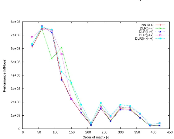
0 1e+08 2e+08 3e+08 4e+08 5e+08 6e+08 7e+08 8e+08

0 50 100 150 200 250 300 350 400 450

Performance [MFlops]

Order of matrix [-]

No DLR DLR(i->j) DLR(i->k) DLR(j->k) DLR(i->j->k)

(18)

1e+08 1.5e+08 2e+08 2.5e+08 3e+08 3.5e+08 4e+08 4.5e+08 5e+08 5.5e+08

0 100 200 300 400 500 600 700

Order of matrix [-]

No DLR DLR(i->j) DLR(i->k) DLR(j->k) DLR(i->j->k)

Fig. 6.Performance ofMMM STDfor Testing configuration 2.

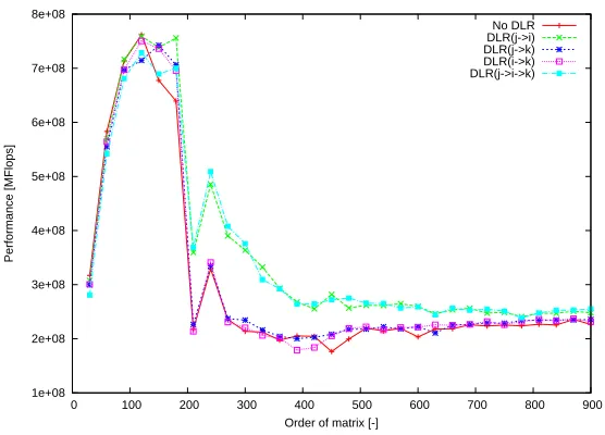
1e+08 2e+08 3e+08 4e+08 5e+08 6e+08 7e+08 8e+08

0 100 200 300 400 500 600 700 800 900

Order of matrix [-]

No DLR DLR(j->i) DLR(j->k) DLR(i->k) DLR(j->i->k)

Fig. 7.Performance ofCHF STDfor Testing configuration 1.

The graphs in Figures 5, 6, 7, and 8 illustrate the performance with or without DLR. These graphs illustrate that DLR increases the code performance due to better cache

uti-lization. There is a performance gap (e.g. for n = 210for the CHF STD for Testing

(19)

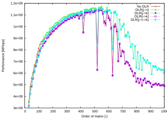
3e+08 4e+08 5e+08 6e+08 7e+08 8e+08 9e+08 1e+09 1.1e+09 1.2e+09

0 100 200 300 400 500 600 700 800 900 1000

Order of matrix [-]

No DLR DLR(j->i) DLR(j->k) DLR(i->k) DLR(j->i->k)

Fig. 8.Performance ofCHF STDfor Testing configuration 2.

0 0.01 0.02 0.03 0.04 0.05 0.06 0.07 0.08 0.09

0 100 200 300 400 500 600 700 800 900

Cache miss ratio [-]

Order of matrix [-]

L2 cache L1 cache Performance

Fig. 9.Study of impact of cache utilization on performance ofCHF STDfor Testing configuration 1.

The graphs in Figures 9, and 10 illustrate the impact of cache utilization on the

per-formance ofCHF STD(the numbers of cache misses are measures by the software cache

(20)

0 0.01 0.02 0.03 0.04 0.05 0.06 0.07

0 100 200 300 400 500 600 700 800 900

Cache miss ratio [-]

Order of matrix [-] L2 cache

L1 cache Performance

Fig. 10.Study of impact of cache utilization on performance ofCHF STDfor Testing configura-tion 2.

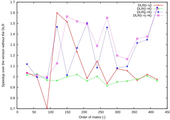
0.7 0.8 0.9 1 1.1 1.2 1.3 1.4 1.5 1.6 1.7

0 50 100 150 200 250 300 350 400 450

Speedup over the version without the DLR

Order of matrix [-]

DLR(i->j) DLR(i->k) DLR(j->k) DLR(i->j->k)

Fig. 11.Speedup ofMMM STDfor Testing configuration 1.

arise due to the other reasons (translation lookaside buffer misses, unsuccessful compiler optimizations, etc.).

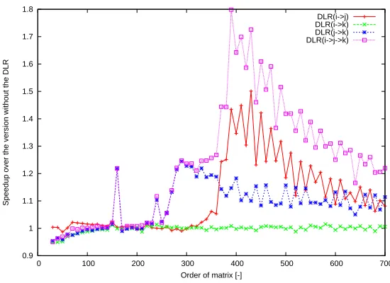
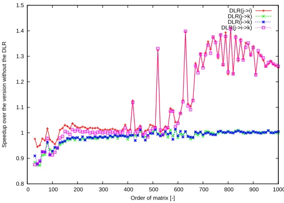
The graphs in Figures 11, 12, 13, 14, 15, and 16 show the speedup over the version

(21)

0.9 1 1.1 1.2 1.3 1.4 1.5 1.6 1.7 1.8

0 100 200 300 400 500 600 700

Order of matrix [-]

DLR(i->j) DLR(i->k) DLR(j->k) DLR(i->j->k)

0.9 1 1.1 1.2 1.3 1.4 1.5

400 600 800 1000 1200 1400 1600 1800 2000

Order of matrix [-]

DLR(i->j) DLR(j->k) DLR(i->j->k)

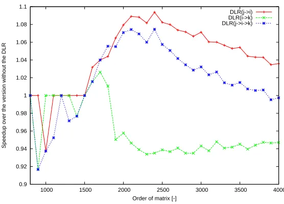
for theMMM STDcode and with DLR(j → i → k) for theCHF STDcode (for Testing

configuraton 1 and 2), and with DLR(j → i) for theCHF STDcode (for Testing

con-figuraton 4) . We can also conclude that the measured speedup is more than 20% in the

(22)

0.8 0.9 1 1.1 1.2 1.3 1.4 1.5 1.6 1.7 1.8

0 100 200 300 400 500 600 700 800 900

Order of matrix [-]

DLR(j->i) DLR(j->k) DLR(i->k) DLR(j->i->k)

Fig. 14.Speedup ofCHF STDfor Testing configuration 1.

0.8 0.9 1 1.1 1.2 1.3 1.4 1.5

0 100 200 300 400 500 600 700 800 900 1000

Order of matrix [-]

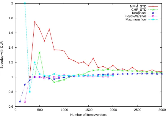
The graphs in Figures 17 and 18 show the speedups over the version without DLR.

We can conclude that DLR can accelerateKP STD,FW STD, andMF STDcodes.

(23)

0.9 0.92 0.94 0.96 0.98 1 1.02 1.04 1.06 1.08 1.1

1000 1500 2000 2500 3000 3500 4000

Order of matrix [-]

DLR(j->i) DLR(i->k) DLR(j->i->k)

0.9 1 1.1 1.2 1.3 1.4 1.5 1.6

0 500 1000 1500 2000 2500 3000

Speedup with DLR

Number of items/vertices

Knapsack Floyd-Warshall Maximum flow

Fig. 17.Speedup ofKP STD,FW STD, andMF STDalgorithms for Testing configuration 3.

6.2. Cache miss rate evaluation

The cache utilization is enumerated according to the following definitions.

Relative number of cache misses= the number of cache misses with DLR

(24)

0.6 0.8 1 1.2 1.4 1.6 1.8 2

0 500 1000 1500 2000 2500 3000

Speedup with DLR

Number of items/vertices

MMM_STD CHF_STD Knapsack Floyd-Warshall Maximum flow

Fig. 18.Speedup ofMMM STD,CHF STD,KP STD,FW STD, andMF STDalgorithms for Testing configuration 4.

The graphs on Figures 19, 20, 21, and 22 illustrate the number of cache misses

occur-ring duoccur-ring one execution of theMMM STDorCHF STDpseudocodes. We can conclude

that

– a DLR effect depends on the value of the parameternand on the cache memory size

(this observation proves the results of the analytical model from Section 4.3)

– except for few cases, where the DLR transformation has a positive impact on cache

utilization.

6.3. Evaluation of a simplified RD model based on GRD

Analytical cache model forMMM STD To analyse this algorithm, we omit the accesses

in an arrayCat a code line (6), because they are much less frequent. In this simplified

model, the algorithm contains the following types of memory accesses:

– If DLR(i→j) is applied, then memory operations withA[i][k]are of the typeβand

memory operations withB[k][j]are of the typeα.

– If DLR(j→k) is applied, then memory operations withA[i][k]are of the typeαand

memory operations withB[k][j]are of the typeδ.

Analytical cache model forCHF STD For analysing this algorithm, we omit the memory

accesses outside thek-loop at a code line (8), because their contributions are negligible.

(25)

0.4 0.5 0.6 0.7 0.8 0.9 1 1.1 1.2

0 100 200 300 400 500 600 700 800 900

Relative number of L1 cache misses [-]

Order of matrix [-]

DLR(i->j) DLR(j->k) DLR(i->k) DLR(i->j->k)

Fig. 19.Relative number of cache misses duringMMM STDfor the L1 cache for Testing configura-tion 1.

0.4 0.5 0.6 0.7 0.8 0.9 1 1.1 1.2 1.3

0 100 200 300 400 500 600 700 800 900

Order of matrix [-]

DLR(i->j) DLR(j->k) DLR(i->k) DLR(i->j->k)

Fig. 20.Relative number of cache misses duringMMM STDfor the L2 cache for Testing configura-tion 1.

– If DLR(j→i) is applied, then memory operations withA[i][k]are of the typeαand

(26)

0.3 0.4 0.5 0.6 0.7 0.8 0.9 1 1.1

0 100 200 300 400 500 600 700 800 900

Order of matrix [-]

Fig. 21.Relative number of cache misses duringCHF STDfor the L1 cache for Testing configura-tion 1.

0.3 0.4 0.5 0.6 0.7 0.8 0.9 1 1.1

0 100 200 300 400 500 600 700 800 900

Order of matrix [-]

Fig. 22.Relative number of cache misses duringCHF STDfor the L2 cache for Testing configura-tion 1.

– If DLR(k→i) is applied, then memory operations withA[i][k]are of the typeγand

(27)

Analytical cache model for spMMM CSR,KP STD, and MF STD The analysis of the cache behavior and DLR effects for these algorithms are beyond the scope of the compiler due to its irregular memory pattern.

Example of the evaluation of the cache analytical model We apply DLR(j→k) on the MMM STDpseudocode. In this case as we stated above, memory operations withA[i][k]

are of the typeαand memory operations withB[k][j]are of the typeδ.

Firstly, we must count how many iterations of thej-loop can reside in the cache. From

the types of memory operations (Eq. (2) on Page 1392), we can derive that

SCMO(A[i][k]) =SD/BS, PDLR(A[i][k]) = 1.

SCMO(B[k][j]) = 1, PDLR(B[k][j]) = 1−SD/BS.

So, the number of iterations is (from the cache parameters in Eq. (1) on Page 1392)

Niter=

DCS BS(1 +SD/BS)

.

The number of cache misses saved by DLR(k, j) per one iteration of thej-loop (Eq. (4)

on Page 1392) isµsaved=Niter.

The total number of cache misses saved by DLR(j→k) during one execution of the

MMM STDpseudocode is

totalµsaved=n2Niter.

For the given cache configuration, it gives the following results

– for Testing configuration 1:

• for L1 cache:Niter= 228.

– for Testing configuration 2:

The discussion on the precision of the simplified RD model Comparisons of the num-bers of estimated and measured cache misses are shown in Figures 23, 24, 25, 26, and 27. Our analytical model is derived from GRD which is based on a fully-associative cache memory assumption. This assumption is the main source of errors in predictions. The errors are higher for the caches with low associativity (e.g. the direct-mapped cache in Testing configuration 5a, Figure 25). On the other hand, our model is relatively precise (e.g. the caches in Testing configuration 5b or 5c, Figures 26 and 27) for caches with

higher associativity (i.e.,s≥4). This condition is true for the majority of modern CPU

(28)

-1e+07 0 1e+07 2e+07 3e+07 4e+07 5e+07 6e+07 7e+07 8e+07 9e+07

0 100 200 300 400 500 600 700 800 900

Number of saved L1 cache misses [-]

Order of matrix [-] Measured

Predicted

Fig. 23.Comparison of the numbers of estimated and measured cache misses (µsaved) saved by DLR during the execution ofMMM STDfor the L1 cache.

-1e+07 0 1e+07 2e+07 3e+07 4e+07 5e+07 6e+07 7e+07 8e+07 9e+07 1e+08

0 100 200 300 400 500 600 700 800 900

Order of matrix [-] Measured

Predicted

Fig. 24.Comparison of the numbers of estimated and measured cache misses (µsaved) saved by DLR during the execution ofMMM STDfor the L2 cache.

6.4. Evaluation of the combination of DLR and loop tiling

We have also measured the performance and cache utilization for the pseudocodeMMM TIL

(29)

-1e+07 0 1e+07 2e+07 3e+07 4e+07 5e+07 6e+07 7e+07

200 400 600 800 1000 1200 1400 1600 1800 2000

Order of matrix [-] Measured DLR(j->k)

Measured DLR(i->j) Predicted DLR(j->k) Predicted DLR(i->j)

Fig. 25.Comparison of the numbers of estimated and measured cache misses (µsaved) saved by DLR during the execution ofMMM STDfor Testing configuration 5a).

0 1e+07 2e+07 3e+07 4e+07 5e+07 6e+07 7e+07

200 400 600 800 1000 1200 1400 1600 1800 2000

Fig. 26.Comparison of the numbers of estimated and measured cache misses (µsaved) saved by DLR during the execution ofMMM STDfor Testing configuration 5b).

(30)

-5e+08 0 5e+08 1e+09 1.5e+09 2e+09 2.5e+09 3e+09 3.5e+09 4e+09 4.5e+09

200 400 600 800 1000 1200 1400 1600 1800 2000

Fig. 27.Comparison of the numbers of estimated and measured cache misses (µsaved) saved by DLR during the execution ofMMM STDfor Testing configuration 5c).

from the optimal value. When DLR is applied, the growth is more smooth, so the code is less sensitive to the tiling factor value. Hence, the DLR technique is useful in the cases when it is hard to predict a good value for the tiling factor.

6.5. Evaluation of DLR for thespMMM CSRcode

ThespMMM CSRcode is a simple example of an irregular code. In this code, the memory access pattern is hard to predict on the compiler level and loop tiling is excluded. But DLR is usable and the application of this technique can save a reasonably large number of the cache misses (see Figures 30, 31, and 32). The numbers of L1 cache misses remain the same (without and with DLR), so graphs are shown only for the L2 cache utilization.

7. Automatic compiler support of DLR

The DLR transformation brings new possibilities to optimize the nested loops.

7.1. Proposed algorithm of an automatic compiler support of DLR

We assume that the optimizing compiler evaluates each loop nest (for details see [33])

independently. LetL1...brepresent ab-dimensional loop nest (hierarchy of immediately

nested loops), whereL1is the outermost loop andLbis the innermost loop. The control

variable for the loopLiis denoted asCi. We propose the following function that returns a

(31)

0 0.02 0.04 0.06 0.08 0.1

0 20 40 60 80 100

L1 cache miss rate [-]

Tile size [-] no DLR DLR(j->k) DLR(i->j) DLR(i->j->k) (a) 0 0.1 0.2 0.3 0.4 0.5 0.6

0 200 400 600 800 1000 1200

Tile size [-]

no DLR DLR(j->k) DLR(i->j) DLR(i->j->k)

(b)

Fig. 28.The L1 miss rate for anMMM TILalgorithm (forn=1024) for small and large values of the tile size. 0 0.002 0.004 0.006 0.008 0.01

0 50 100 150 200

Tile size [-] no DLR DLR(j->k) DLR(i->j) DLR(i->j->k) (a) 0 0.01 0.02 0.03 0.04 0.05 0.06 0.07 0.08

0 200 400 600 800 1000

Tile size [-] no DLR

DLR(j->k) DLR(i->j) DLR(i->j->k)

(b)

Fig. 29.The L2 miss rate for anMMM TILalgorithm (forn=1024) for small and large values of the tile size.

1: procedureDLR APPLICATION(inb,L,C;outres)

2: res= [];

3: fori←1, b−1do .here we consider application of DLR(Ci → Ci+1)

4: ifthis DLR application is possiblethen .i.e., loopLi+1is reversible

5: computeµsavedfrom the proposed cache model;

6: compute overhead of this DLR application;

7: ifthis DLR application pays-offthen

8: addito theres;

9: returnres;

If this function returns an empty list (in variableres), then DLR does not pay off for

any loop in loop nest L. In another case, it returns a list (in variable res) of the loop

(32)

0 0.01 0.02 0.03 0.04 0.05 0.06 0.07 0.08

0 1000 2000 3000 4000 5000 6000

Order of matrices [-]

no DLR DLR(y->i->j)

Fig. 30. The L2 cache miss rate for an spMMM CSR algorithm (for density(A) = 7% and density(B) = 21%)

the code performance. In real applications, the benefits of DLR application should be compared to the other source code optimizations.

7.2. Discussion on the DLR applicability inside the compilers

The function in Section 7.1 is very brief. The compiler optimization must address more issues:

– Where can DLR be applied? DLR can be applied on all nested reversible loops

(ex-cluding outermost loops). This condition can be easily checked by the compiler.

– Where should DLR be applied? DLR should be applied on a pair or triple of loops,

which causes a maximal effect on cache behavior (mentioned in Section 3.3). This compiler decision is very similar as the one for the loop tiling.

– Does DLR have a significant effect? Yes. In most cases, higher speedups are achieved

by the loop unrolling or loop tiling. But DLR can be combined with these techniques (see Section 6.4), and moreover, it can be applied on the codes, where the application of the loop tiling is not possible (see Section 6.5).

– Is DLR supported in any compiler system? No, providing an automatic support of

(33)

0.056 0.058 0.06 0.062 0.064 0.066 0.068 0.07

0 5 10 15 20 25 30 35 40

Density of matrix A [%]

no DLR DLR(y->i->j)

Fig. 31.The L2 cache hit rate for an algorithmspMMM(forn=2200 anddensity(B) = 17%)

• The DLR pays off for the majority of measured situations, but the exact threshold

depends strongly on the measured problem and also on the exact configuration for the measurement. The model of the cache behavior is introduced, but it can predict the number of “saved”cache misses only for some types of accesses (this model is unusable e.g. for the indirect access etc.)

• The presented model can predict “saved”cache misses, but the DLR

transforma-tion also increases the number of conditransforma-tional branches. Furthermore, effects of these cache misses or conditional branches are influenced by the other compiler optimizations.

• The explicit use of DLR can confuse optimizing compilers and hinder further

loop optimizations (since it “destroys”perfectly nested loops etc.). So, it should be applied as the last possible high-level optimization.

8. Conclusions

We have described a new code transformation technique, the dynamic loop reversal, whose goal is to improve the locality of the accessed data and improve the cache uti-lization. This transformation seems to be very useful for the codes with nested loops. We have demonstrated significant performance gains for six basic algorithms from linear algebra, graph theory etc.

We have also developed a probabilistic analytical model for this transformation and compared the numbers of measured cache misses and the numbers of cache misses es-timated by the model. The inaccuracies of the model occur mainly due to the fully-associative cache memory assumption.

(34)

0.05 0.052 0.054 0.056 0.058 0.06 0.062 0.064

0 5 10 15 20 25 30 35 40

Density of matrix B [%]

no DLR DLR(y->i->j)

Fig. 32.The L2 cache hit rate for an algorithmspMM(forn=3700 anddensity(A) = 10%)

Acknowledgments.This work was supported by RVO|18000|ext:|FIS:110−111000|grant of M ˇSMT.

References

1. Ahmed, N., Mateev, N., Pingali, K.: Tiling imperfectly-nested loop nests. In: Proceedings of the 2000 ACM/IEEE conference on Supercomputing (CDROM). SC ’00, IEEE Computer Society, Washington, DC, USA (2000), http://dl.acm.org/citation.cfm?id=370049. 370401

2. Anderson, E., Bai, Z., Bischof, C., Blackford, L.S., Demmel, J., Dongarra, J., Croz, J.D., Greenbaum, A., Hammarling, S., McKenney, A., Sorensen, D.: LAPACK user’s guide (1999),

http://epubs.siam.org/doi/abs/10.1137/1.9780898719604

3. Beyls, K.: Exact compile-time calculation of data cache behavior. http://www.elis. rug.ac.be/aces/edegem2002/beyls.pdf

4. Beyls, K., D’Hollander, E.: Reuse distance as a metric for cache behavior. In: Proceedings of PDCS’01. pp. 617–662 (August 2001),citeseer.ist.psu.edu/beyls01reuse. html

5. Carr, S., Kennedy, K.: Blocking linear algebra codes for memory hierarchies. In: Proceedings of the Fourth SIAM Conference on Parallel Processing for Scientific Computing. pp. 400– 405. Society for Industrial and Applied Mathematics, Philadelphia, PA, USA (1990),http: //dl.acm.org/citation.cfm?id=645819.669407

6. Carr, S., Lehoucq, R.: Compiler blockability of dense matrix factorizations. ACM Transactions on Mathematical Software 23, 336–361 (1996)

(35)

8. Datta, K., Murphy, M., Volkov, V., Williams, S., Carter, J., Oliker, L., Patterson, D., Shalf, J., Yelick, K.: Stencil computation optimization and auto-tuning on state-of-the-art multi-core architectures. In: Proceedings of the 2008 ACM/IEEE Conference on Supercomputing. pp. 4:1–4:12. SC ’08, IEEE Press, Piscataway, NJ, USA (2008),http://dl.acm.org/ citation.cfm?id=1413370.1413375

9. Dongarra, J.J., Croz, J.D., Hammarling, S., Duff, I.: A set of level 3 Basic Linear Algebra Subprograms. ACM Transactions on Mathematical Software 16(1), 1–17 (Mar 1990)

10. Golub, G.H., Van Loan, C.F.: Matrix Computations (3rd ed.). Baltimore: Johns Hopkins (1996) 11. Im, E.: Optimizing the Performance of Sparse Matrix-Vector Multiplication - dissertation

the-sis. University of California at Berkeley (2001)

12. ˇSimeˇcek, I., Tvrd´ık, P.: Sparse matrix-vector multiplication — final solution? In: Paral-lel Processing and Applied Mathematics. PPAM’07, vol. 4967, pp. 156–165. Springer-Verlag, Berlin, Heidelberg (2008), http://www.springerlink.com/content/ 48x1345471067304/

13. ˇSimeˇcek, I., Tvrd´ık, P.: Dynamic loop reversal — the new code transformation technique. In: Ganzha, M., Maciaszek, L.A., Paprzycki, M. (eds.) Federated Conference on Computer Science and Information Systems (FedCSIS). pp. 1587–1594 (2013)

14. John L. Hennessy, D.A.P.: Computer Architecture, Fourth Edition: A Quantitative Approach. Morgan Kaufmann; 4 edition (September 27, 2006) (2006), http://www.amazon. com/Computer-Architecture-Fourth-Quantitative-Approach/dp/

0123704901/ref=pd_sim_b_1

15. Kennedy, K., Allen, J.R.: Optimizing compilers for modern architectures: a dependence-based approach. Morgan Kaufmann Publishers Inc. (2002)

16. Klint, P., van der Storm, T., Vinju, J.: Rascal: A domain specific language for source code analysis and manipulation. In: Source Code Analysis and Manipulation, 2009. SCAM ’09. Ninth IEEE International Working Conference on. pp. 168–177 (Sept 2009)

17. Mernik, M., Heering, J., Sloane, A.M.: When and how to develop domain-specific languages. ACM Comput. Surv. 37(4), 316–344 (Dec 2005), http://doi.acm.org/10.1145/ 1118890.1118892

18. Press, H.W., Teukolsky, S.A., Vetterling, W.T., Flannery, B.P.: Numerical Recipes: The Art of Scientific Computing. Cambridge University Press (2007)

19. Seward, J., Nethercote, N., Hughes, T., Fitzhardinge, J., Weidendorfer, J., Mackerras, P., et al.: Valgrind documentation, http://valgrind.org/docs/manual/valgrind_ manual.pdf

20. Song, Y., Li, Z.: New tiling techniques to improve cache temporal locality. SIGPLAN Not. 34, 215–228 (May 1999),http://doi.acm.org/10.1145/301631.301668

21. Tang, Y., Chowdhury, R.A., Kuszmaul, B.C., Luk, C.K., Leiserson, C.E.: The pochoir sten-cil compiler. In: Proceedings of the Twenty-third Annual ACM Symposium on Parallelism in Algorithms and Architectures. pp. 117–128. SPAA ’11, ACM, New York, NY, USA (2011),

http://doi.acm.org/10.1145/1989493.1989508

22. Tuma, M.: Overview of direct methods. I. Winter School of SEMINAR ON NUMERICAL ANALYSIS (January 2004)

23. Tvrd´ık, P., ˇSimeˇcek, I.: Analytical modeling of optimized sparse linear code. In: Parallel Pro-cessing and Applied Mathematics. vol. 3019/2004, pp. 207–216. Czestochova, Poland (2003),

http://www.springerlink.com/content/drwdhen7db199k05/

24. Tvrd´ık, P., ˇSimeˇcek, I.: Analytical model for analysis of cache behavior during cholesky fac-torization and its variants. In: Proceedings of the International Conference on Parallel Pro-cessing Workshops (ICPP 2004). vol. 12, pp. 190–197. Montreal, Canada (2004), http: //dl.acm.org/citation.cfm?id=1018426.1020360

(36)

and Applied Mathematics. PPAM’05, vol. 12, pp. 164–171. Springer-Verlag, Poznan, Poland (2005),http://dl.acm.org/citation.cfm?id=2096870.2096894

26. Tvrd´ık, P., ˇSimeˇcek, I.: Software cache analyzer. In: Proceedings of Czech Technical University Workshop. vol. 9, pp. 180–181. Prague, Czech Republic (mar 2005)

27. Vera, X., Xue, J.: Efficient compile-time analysis of cache behaviour for programs with IF state-ments. In: International Conference on Algorithms And Architectures for Parallel Processing. pp. 396–407. Beijing (October 2002),citeseer.ist.psu.edu/567600.html

28. Vera, X., Xue, J.: Let’s study whole-program cache behaviour analytically. In: Proceedings of the 8th International Symposium on High-Performance Computer Architecture. pp. 175–186. HPCA ’02, IEEE Computer Society, Washington, DC, USA (Feb 2002),http://dl.acm. org/citation.cfm?id=874076.876456

29. Vuduc, R., Demmel, J.W., Yelick, K.A., Kamil, S., Nishtala, R., Lee, B.: Performance opti-mizations and bounds for sparse matrix-vector multiply. In: Proceedings of Supercomputing 2002. Baltimore, MD, USA (November 2002)

30. Wadleigh, K.R., Crawford, I.L.: Software optimization for high performance computing. Hewlett-Packard professional books (2000)

31. Wolf, M.E., Lam, M.S.: A data locality optimizing algorithm. SIGPLAN Not. 26, 30–44 (May 1991),http://doi.acm.org/10.1145/113446.113449

32. Wolfe, M.: High-Performance Compilers for Parallel Computing. Addison-Wesley, Reading, Massachusetts, USA (1995)

33. Xue, J.: Loop tiling for parallelism. Kluwer Academic Publishers, Norwell, MA, USA (2000)

Ivan ˇSimeˇcek 2009-now Assistant Professor at the Department of Computer Systems, Faculty of Information Technology, Czech Technical University in Prague (CTU in Prague). 2009-now Executive manager of the Prague Nvidia CUDA teaching center.

* Author of more than 40 scientific journals and conference publications.

* Main research areas: GPGPU, distributed algorithms, sparse matrix storage formats, numerical linear algebra, cache memory models, programming languages, applied crys-tallography.

Pavel Tvrd´ık2009–now professor, Department of Computer Systems, FIT CTU in Prague. 2009–now dean, FIT CTU in Prague.

2009-now member of scientific councils of FIT CTU in Prague

* Author or co-author of 10 papers in journals in WoS and over 50 papers in proceedings of refereed conference proceeding. Co-editor of 1 book in IEEE Computer Science Press. Documented over 65 citations in WoS.

* A member of editorial board of Scalable Computing: Practice and Experience (since 2005).

* Member of IPCs of more than 50 international conferences, including: ICCS’11, PDCN’11, PDCS’11, HPCS’10, LaSCoG-SCoDiS’10, PDCN’10, ICCS’10, PPAM’09, PDCS’09, PDCN’09, ICCS’09, PDCS’08, PDCN’08, ICCS’08, PDCN’07, ICCS’07, PPAM’07, PDCS’07, HPCS’07, ICCSA’07, PDCS’06, PDCN’06, InfoScale’06, ICCS’06, ICCSA’06.

* Main research areas: Parallel architectures and algorithms, programming languages.