1 2 3 4 5 6 7 8 9 10 11 12 13 14 15 16 17 18 19 20 21 22 23 24 25 26 27 28 29 30 31 32 33 34 35 36 37 38 39 40 41 42 43 44 45 46 47 48 49 50 51 52 53 54 55 56 57 60
An Economic Side-Effect for Pre
fi
x Deaggregation
Andra Lutu
Institute IMDEA Networks, Spain University Carlos III of Madrid, Spain
Marcelo Bagnulo
University Carlos III of Madrid, Spain
Rade Stanojevic
Institute IMDEA Networks, Spain University Carlos III of Madrid, SpainAbstract—The injection of artificially fragmented prefixes through BGP is a widely used traffic engineering technique. In this paper we examine one particular economic side-effect of deaggregation, namely the impact on the transit traffic bill. We show that the use of more-specific prefixes has a traffic stabilization side-effect which translates into a decrease of the transit traffic bill. We propose an analytical model in order to quantify the impact of deaggregation on the transit costs. We validate our results by means of simulations and through the extensive analysis of real BGP routing information data.
Index Terms—BGP, Economics, Modeling, Traffic Engineering
I. INTRODUCTION
The Internet is the interconnection of over 36000domains known as Autonomous Systems (ASes), which engage in dynamic relationships that interplay with their technical and economic necessities. The routing between ASes relies on the Border Gateway Protocol (BGP), which is responsible for the exchange of reachability information and the selection of paths according with the policies specified by each domain.
The way in which the traffic flows in the interdomain is influenced by the path dynamics triggered in the continuous evolution of the Internet topology and the routing policies of each network. Hence, individual network managers need to permanently adapt to the interdomain routing changes and, by engineering the Internet traffic, optimize the use of their network. One important task achieved through the use of traffic engineering tools is the control and optimization of the routing function in order to allow the ASes to shift the incoming and outgoing traffic in the most effective way.
The injection of more-specific prefixes through BGP rep-resents a powerful traffic engineering tool which offers a
fine-grained method to control the interdomain ingress traffic. This technique implies that ASes selectively announce dis-tinct fragments of their address block to different upstream providers. This type of phenomenon is commonly known as
prefix deaggreagation. The most important negative side-effect of the widespread adoption of this technique is the artificial inflation of the BGP routing table [1], which can affect the scalability of the global routing system.
In this paper we study the impact of address-space fragmen-tation on the transit bill of the networks originating the more-specific prefixes. As a result of the unique interaction between the path changes in the current Internet [2], the distribution of traffic on sources and the widely used95th percentile billing
method [3], [4], we find that the deaggreagating ASes enjoy one particular benefit from fragmenting their address space:
the decrease of the transit traffic bill. We propose an Internet model to analyze the cost for transit in two extreme cases of deaggreation, i.e. no deaggregation and full deaggregation1.
We demonstrate that by using deaggreagation and scoped advertisements, the originating AS reduces the path diversity towards the injected prefixes. Thus, the amount of traffic destined to a particular sub-block of addresses is bound to the incoming link on which it was injected. This eliminates the possibility for any trafficfluctuations due to routing changes towards that particular prefix. Since the transit bill depends on the peak traffic usage and not on the total traffic usage, avoiding trafficfluctuations implies a lower monthly bill.
We begin, in section II, by explaining the intuition behind the network dynamics captured in the paper through the analysis of a toy example. We continue by presenting in section III the general model used for quantifying the effect of different deaggregating strategies on the ASes’ transit costs. In section IV we estimate the model parameters by performing an extensive analysis of real BGP routing information. We afterwards quantify the actual impact of deaggregation. We further contrast the model-generated results with simulation and data-driven results. Finally, we conclude the paper in section V and present directions for future work.
II. TOYEXAMPLE
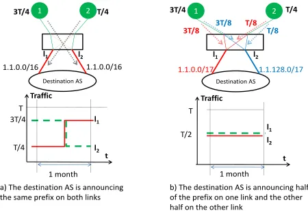
In order to provide the intuition behind the BGP phenomena modeled and analyzed in this paper, let us consider the simple case of one destination network announcing the same prefix
1.1.0.0/16 over two different transit links, like we can see in Figure 1.a. For this toy example, we reduce the number of sources in the interdomain to only two, out of which one is generating 34 of the whole trafficT consumed by the destination network, and the other one, the rest.
We monitor the traffic on each transit link during one month. We consider that the 3T
4 source AS is sending its traffic on link
l1for half of the period, after which, due to a routing change, it starts forwarding its traffic on link l2. The T4 source AS suffers the opposite events, namely it sends the traffic during the first half of the month through linkl2 and for the second half of the month it switches to linkl1. The transit traffic cost is calculated using the95thpercentile rule for each of the two
links. As a result, because the traffic on linkl1 had a level of 3T
4 for more than 5%of the billing period, the transit traffic
1We definefull deaggregationas splitting the address block into as many
1 2 3 4 5 6 7 8 9 10 11 12 13 14 15 16 17 18 19 20 21 22 23 24 25 26 27 28 29 30 31 32 33 34 35 36 37 38 39 40 41 42 43 44 45 46 47 48 49 50 51 52 53 54 55 56 57 60
1 2
Destination AS
3T/4 T/4
t Traffic
T 3T/4
T/4
1 month l2
l1
1 2
Destination AS
3T/4 T/4
t Traffic
T
T/2
1 month l2
l1
l2
l1
l1
l2
a) The destination AS is announcing the same prefix on both links
b) The destination AS is announcing half of the prefix on one link and the other half on the other link
3T/8 3T/8 T/8 T/8
1.1.0.0/16 1.1.0.0/16 1.1.0.0/17 1.1.128.0/17
Fig. 1. Toy example representation.
bill for linkl1isc34T. Similarly, the transit traffic bill for link
l2is alsoc34T, because for more than5%of the billing period the traffic level was 3T
4 . Therefore, the total cost payed for the consumed trafficT isc3T
2 , which is withcT2 higher than the cost cT paid based on the 95th percentile rule if no routing
changes would happen.
We show in this paper that the destination AS can avoid the fluctuations of traffic due to routing changes through deaggregation and thus also avoid the implicit augmentation in the transit traffic monthly bill. Consider that the desti-nation AS divides its address space into two more-specific prefixes and announces each on a separate link, i.e. announces 1.1.0.0/17 through link l1 and 1.1.128.0/17 through link l2, like we can observe in Figure 1.b. This means that no traffic
fluctuations induced by routing dynamics exist on either links and, consequently, the sum of the95th percentiles on the two
links is simply T. Consequently, in this scenario, the routing changes cannot impact the95thpercentile and the transit traffic
monthly bill for the destination AS iscT.
Regardless of the simplicity of the example presented here, the toy model does illustrate the basic intuition behind the observed phenomena, where routing changes may increase the transit bill for the destination AS, without increasing its total incoming traffic. In the following section, we propose the general Internet model which extends this example to capture more complex aspects of the Internet.
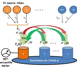
III. MODELDESCRIPTION ANDSAVINGSANALYSIS The general Internet model described here accounts for the route dynamics which are responsible for large traffic shifts in the interdomain, like previously observed in [2]. Given that, in the current Internet, paths are calculated independently for each destination, we model the Internet at the AS-level assuming, without any loss of generality, the existence of one destination AS and N sources of traffic. We perform our analysis on the case of the destination network with n
links accommodating the incoming traffic from N sources. We assume a symmetric model where all the links have the same capacity.For the ease of the presentation, we assume an uniform distribution of incoming traffic on the destination address space. In the case of an uneven traffic distribution, it
1 . . . .
AS rank
Origina
ted
tr
af
fi
c Traffic generated by
the N source Ases: Zipf distribution
n transit links Routing:
sticky model
Destination AS Prefix p
Billing: 95th percentile
rule
. . . .
2 3 j N
t1 t2
t3 t
j t
N
Fig. 2. Graphical representation of the proposed Internet model for routing changes.
can be easily proved that a correspondingly proportional prefix fragmentation can be found so that the amount of traffic per more-specific prefix are comparable. As depicted in Figure 2, we integrate here three important elements, i.e. the interdomain path changes, the traffic model and the cost model. Their entanglement offers the necessary structure for studying the influence of deaggreagation techniques on interdomain traffic.
A. Deaggregation Strategies and The Sticky Model for Inter-domain Routing Changes
We model two extreme behaviours with respect to prefix deaggregation. We denote byλthe number of prefixes injected in the interdomain by the origin AS. One behaviour describes the AS which can choose to announce the same aggregated prefix through all its links (λ = 1). Alternatively, the origin AS can decide to evenly fragment its address block across its providers and announce disjoint more-specific prefixes on different transit links (λ= n). We assume that the assigned address space can be evenly split between the available number of links and announced by the destination AS as a single more-specific prefix separately on a different link2. Moreover, we
assume that the announced prefixes are propagated as injected by the origin [5], which is aligned with current operational practices. Additionally, we assume the full reachability of the injected prefixes, meaning that every AS in the interdomain receives several routes for thenprefixes corresponding to the originating AS and selects one route for each prefix. In order to better understand the impact of the path changes on the cost for transit traffic, we analyze the path changes in a period of time relevant for the billing process, namely a month.
We model the interdomain route dynamics as follows. We model the initial-state set of routes as a random selection between the available BGP paths between each source AS towards any destination prefix, performed at the beginning of the analyzed time interval. In other words, we assume that if
2While it is not always true that the evenly divided address space can be
1 2 3 4 5 6 7 8 9 10 11 12 13 14 15 16 17 18 19 20 21 22 23 24 25 26 27 28 29 30 31 32 33 34 35 36 37 38 39 40 41 42 43 44 45 46 47 48 49 50 51 52 53 54 55 56 57 60
a destination AS announces a prefix over n different links, then the probability that any of those links is a part of the forwarding path from a source towards the destination at the initial state is 1
n. This assumption can be easily modified so
that the model includes a different probability distribution on the available transit links.
In the rest of the time interval, we analyze the routing state by incorporating the dynamics of the routing process due to topology or policy changes3. We divide the month
into 5 minutes intervals (consistent with the 95th percentile
billing rule) and use a time-slotted model to analyze the impact of path changes. Keeping in mind the fact that the majority of paths in the Internet are usually remarkably stable [6], we surmise in our model a small probability p for the path used in a given time-slot during a month to be different from the initially chosen one. Thus, we consider that the system is constantly performing a sticky process for readjusting to changes in the network.
B. Traffic model
In this section we model the traffic distribution on the avail-able incoming links, depending on the manner the destination AS injects its prefix(es) in the interdomain.
We assume that each source network j included in our model generates an amount of traffic tj towards a given
destination in the interdomain, with the distribution depicted in Figure 2. We assume that the generated traffictj follows a
Gaussian distribution characterized by the statistical mean μj
and a variance σ2
j.
1) Distribution of Traffic on Sources: We assume that the traffic generated towards a given destination is distributed among the existing sources according with Zipf’s law, as previously described in [7]. This assumption is consistent with the traffic measurements in [8], as the Zipf distribution is a particular case of a power law distribution. Given a ranking of the Internet entities, the Zipf law states that the traffic generated by a network is inversely proportional with its rank. For any destination network we assign the following amount of incoming traffic from AS with rankj:
tj=
1
jα
N
k=1k1α
T =zj(α)T, (1)
wherezj(α)is thejranked element corresponding to ASjin
a Zipf distribution ofNelements with the skewness parameter
α. The total amount of traffic received by the destination AS can be expressed as the sum of all the traffic contributions
T =Nj=1tj, for all sourcesj in the Internet.
2) Distribution of Traffic on Transit Links: The total amount of traffic T consumed by a particular AS in the Internet consists of the contribution of all the sources in the interdomain. We analyze here the traffic distribution on then
ingress links of a destination AS.
3We do not consider the routing changes due to ingress link failures, as
these changes cannot be accounted as potential savings since any operational viable deaggregation strategy must support backup links.
Destination AS / Prefix p
1 2 n
T/n
95th
percentile meter
TT--1(t)
TT--n (t) TT--2 (t)
2
1 3 . . . . N-1 N
N source ASes
s1
Tl (t)
. . . . . .
. . .
t1 t2 t3 tN-1 tN
TT+1 (t)
Fig. 3. Traffic dynamics for each transit link.
We begin by characterizing the distribution of traffic on the incoming links of a destination AS that announces its address space as one single aggregated prefix. Consequently, any of the available links towards the destination network can be a part of the traffic forwarding path. For a given destination AS with n links we define the subset si of sources which
have as initial state path a route which includes linki, where
i = 1, n. For example, as depicted in Figure 3, subset s1 includes all the source networks that have chosen transit link
1 in the initial phase of the model. Due to the fact that each link has the same probability of being chosen by each source for traffic forwarding in the initial state of the interdomain routing process, the expected value of the size of source sets
si is of Nn ASes. Consequently, in case of no deaggregation,
the incoming traffic on each link in the initial state of the routing process has an expected value of T
n.
When dividing the month in many equal-sized time-slots, we further consider that the sticky routing model is adapting in each time-slot to the path changes which may have occurred. Therefore, in every time interval in the analyzed period, with a probabilityp the current forwarding path is different from the one used by the same AS in the initial state. This triggers the shift of a certain amount of traffic from linkl to the rest of the links for the destination AS and the other way around. We denote withθ−i (t)the random variable which represents
the traffic reduction at moment t from link i and dividing among the rest of the transit links, as we can observe in Figure 3. The unstable trafficθ−
i (t)leaving link i at moment t can
be further expressed asj∈siqj(t)tj, wheretjrepresents the
traffic generated by source ASjand has the expression in (1),
sirepresents the set of sources with initial-state path including
link i and qj is either 1 if at moment t link i is a part of
AS j’s forwarding path or 0 in the contrary case. Formally,
P(qj = 1) =pandP(qj = 0) = 1−p. The traffic reduction
follows a Binomial distribution, i.e. θ−
i ≈ Binomial(Nn, p),
withi∈[1, n].
When analyzing the traffic on a link we also have to consider
the traffic increasein the current link ifrom receiving traffic from the rest of the links k = i. This represents only a fraction of the total traffic moving away from any other link towards the current transit link. We denote with θk−(t) the traffic leaving any linkk, wherek=i. Similar to the case of linki, we can expressθk−(t)asj∈s
1 2 3 4 5 6 7 8 9 10 11 12 13 14 15 16 17 18 19 20 21 22 23 24 25 26 27 28 29 30 31 32 33 34 35 36 37 38 39 40 41 42 43 44 45 46 47 48 49 50 51 52 53 54 55 56 57 60
is either1or0depending if at momenttlinkiis a part of the forwarding routed used by the source AS or not andtj has the
expression in (1). The traffic shift probability is equal to the probability of path change p, i.e. P(qj = 1) = p. The total
unstable traffic is represented by k=iθ−
k(t). This amount
evenly splits between all the n−1 equiprobable alternative links, including the analyzed linki. Consequently, the expected value of the incoming traffic denoted by θ+
i (t) on link i is
represented by the 1
n−1 part of all the total unstable traffic, i.e. 1
n−1
k=iθ−k(t).
We can now express the total volume of traffic on each link towards the destination, which changes at every time-slot t
like showed in the following expression:
Ti(t) = Tn −θ−
i (t) +θ+i (t), (2)
where θ−
i (t) represents the traffic leaving link i and θ+i (t)
represents the expected value of the traffic shifting from the rest of the links to link i.
Therefore, the expressions for the statistical mean and variance for the total traffic on link i when a single prefix is announced over all the available links are:
σ2
i =p(1−p) ⎡
⎣1− 1
(n−1)2
|si|=Nn
j∈si
t2
j+(n−11)2 N
j=1
t2
j ⎤ ⎦;
μi =Tn. (3)
In the alternative strategy case of full deaggregation, the AS is announcing as many more-specific prefixes as number of transit links. Consequently, the size of the set of sources with a route that includes linkiin the initial state is|si|=N. In other
words, every source AS installs in its routing table a stable path for each transit link for the destination AS. This implies that the traffic shifting from one link to the others is zero and, similarly, the traffic incoming from the rest of the links is also null. Therefore, the variance of the traffic on each link resulting from route changes is σ2
i = 0, as the traffic forwarding paths
are very stable. Consequently, the incoming traffic on each link equal with T
n is confined to the preferred incoming link
and does notfluctuate during the analyzed period.
C. The Cost Analysis
The95thpercentile ruleis currently the most widely-spread
billing method among ISPs [3]. This method usually implies that the agreed billing period (usually a month) is sampled using afixed-sized window, each interval yielding a value that denotes the traffic transferred during that period. The resulting intervals are sorted and the95thpercentile of this distribution
is used for billing [3].
A recent transit cost survey [9] has shown that the price per unit of transfered traffic, denoted here by ct, decreases with
the increase of the expected volume of transit traffic, following a convex dependency. However, this is only true when the increase of the expected amount of traffic is significant i.e. one order of magnitude. In the case where the increase of expected traffic volume is in the same order as the initial traffic
volume, the cost per Mbps remains constant. We expect that the variations in traffic do not change the order of magnitude of the received traffic, therefore we consider the following linear cost function for the transit traffic:C=ct∗V, whereV is the
charging traffic volume (i.e. the95thpercentile of the monthly
traffic) of the destination AS i and ct is the corresponding
transit traffic unit cost. We consider that the total charging traffic volume for any destination AS represents the addition of all the chargeable traffic volumes on each incoming link, and therefore can be expressed as
V = n
i=1
(μi+ 1.96σi), (4)
where n represents the number of incoming links for the destination AS, andμi andσi have the expressions from (3).
Given the fact that the traffic on link l follows a Binomial distribution B(N, p), we can approximate it with a Normal (Gaussian) distributionN(μi, σ2i). The expressionμ+ 1.96σ
from (4) represents the estimation of the95th percentile of a
Normal random variableN(μ, σ2)representing the individual traffic volume on the incoming links.
In order to capture the impact of deaggregation on the transit traffic bill, we evaluate the amount of chargeable traffic in the two previously mentioned cases. We calculate next the total amount of chargeable traffic on each link, i.e. the
95th percentile of the link traffic, when no deaggregation
is performed by the destination AS (vi|λ=1) and when the number of prefixes announced is equal to the number of available links (vi|λ=n):
vi|λ=1= Tn+1.96
p(1−p) j∈si
t2
j+(n−11)2
k=i
j∈sk
t2
j,
vl|λ=n= Tn. (5)
Consequently, after substituting tj with the
expression in (1), the additional traffic on each link γi = γi(p, α, T) = vi|λ=1 − vi|λ=n becomes
γi = 1.96Tp(1−p)j∈sizj2+
1 (n−1)2
k=i
j∈skzj2
where zj = zj(α) represents the Zipf coefficient in (1).
Furthermore, the difference in the total charging traffic volume for the analyzed destination AS with n links can be expressed as the sum of the trafficfluctuations in all the links, yielding the expression for the total volume of additional chargeable traffic:
γ=γ(n, p, α, T) =n i=1
γi(p, α, T). (6)
The savings in transit traffic bill represent the cost c payed for the burstable, unstable traffic, i.e.c=γct. Henceforth, the
saved amount in the transit traffic bill represents a fraction of
1 2 3 4 5 6 7 8 9 10 11 12 13 14 15 16 17 18 19 20 21 22 23 24 25 26 27 28 29 30 31 32 33 34 35 36 37 38 39 40 41 42 43 44 45 46 47 48 49 50 51 52 53 54 55 56 57 60
expression in (6) yields that the relative transit traffic savings are a function of the number of links towards the destination AS, the instability probability pand the skewness parameter
α: RS=f(n, p, α).
IV. NUMERICALRESULTS ANDMODELVALIDATION In this section we first obtain numerical results for the analytical model. We then validate the model by contrasting these results with quantifications from both simulations and data driven estimations using real BGP traces.
In order to apply the proposed model to the current Internet and estimate the potential savings in the transit costs, we need first to assign realistic values to the model parameters, namely, N,n, αand p. Parameter N stands for the number of ASes in the Internet, which is in the order of 36000. The skewness parameter αfor the Zipf distribution on the traffic sources is estimated in the current state of the art [7], [10] to a value of 0,9. As parameter prepresents the probability of a change in the ingress link used by the source ASes to send traffic towards the destination, we estimate it by analyzing the data set containing real BGP routing information. Parameter
nrepresents the number of transit links which we estimate in the next section following the routing data analysis.
A. Data Set
The data set used includes the full BGP routing table snapshots taken every8hours from66different ASes present in the RIPE database [11], during the months of December 2010 until May 2011. This adds up to a total of more than 35000
snapshots of full routing tables, containing the BGP routing information from the 66 analyzed sources towards more than
350000 destination prefixes. We approximate the amount of
traffic generated by each source by extracting from the Zipf distribution of traffic on the36000sources only the elements corresponding to the official ranks for the set of 66 different analyzed sources. We use the official CAIDA ranks assigned based on the data-set from January 2011 [12]. We estimate the number of different transit links per destination by identifying the unique second last-hops4 (2LH) in the paths installed in
the routing tables. Wefind that more than93%of ASes have at most 7transit providers.
B. Estimation of the Instability Probability
In order to estimate the transit link instability probability, we further observe the changes in the 2LHs of the AS paths towards the destination prefixes in the analyzed routing tables. For each source-destination AS pair, we calculate the probability that in a given interval the source AS is not using the link selected in the initial state towards the same prefix. For each of the 66 sources analyzed, we evaluate the relative time the source AS is not using the path announced in thefirst time slot of the analyzed period towards every destination prefix. Next, we match every destination prefix to the originating AS
4Thesecond last-hopis the AS which we see before the destination AS in
theAS-PathBGP attribute and it represents the upstream provider used by
the source to reach the destination.
2 3 4 5 6 7
0.02 0.03 0.04 0.05 0.06 0.07 0.08 0.09
Number of links
Savings proportion
Analytical model Simulation
Real routing data (mean value)
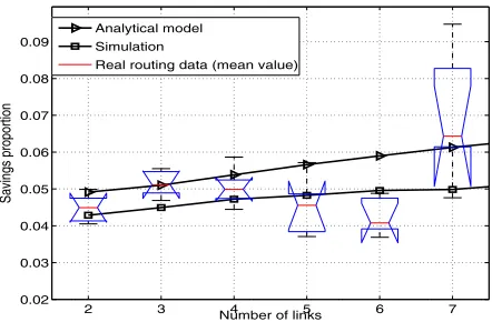
Fig. 4. Model generated, simulation and real-approximation savings curve for a deaggregating AS.
and average the time spent on an alternative path for all the prefixes announced by the destination AS. We thus obtain the probability that a source uses a path towards each destination AS which is different than the initial one. This implies that, for a proportion pof time, traffic may shift from the initial-state transit link towards another of the remaining equiprobable transit links. We approximate the parameterpwith the mean value of the transit link instability probability over all the observed sources, yielding a value ofp= 3.5%.
C. Savings Quantifications using the Analytical Model
We observe in Figure 4 the model savings estimated for a destination AS depending on the number of links. We consider an instability probability ofp= 3.5%in the interdomain and a Zipf distribution of traffic with 36000 elements andα= 0.9. We observe that a destination AS with n∈[2,7]transit links may have an additional cost incurred by the route instabilities in the interdomain that can reach up to 6.5% of the transit traffic. According with the results presented in Figure 4, the average value of the savings for an AS with 2 transit links, representing 40%of all the ASes, is equal with 4.9% of the usual transit traffic bill.
D. Model Validation through Simulation
In order to check the accuracy of the results obtained ana-lytically, we simulate the proposed model for a destination AS withn∈[2,7]transit links. We consider that the destination AS receives traffic from 36000 source ASes, following a Zipf distribution with skewness parameter α = 0.9. We evenly divide the Internet traffic signal in 100 equal-sized time-slots for which we define the sample value of the traffic level, which is consistent with the number of routing snapshots we have during a month. We consider that in the first time-interval, each source AS uniformly chooses one of thenproviders. In the remaining time-slots we simulate the sticky BGP selection algorithm by conceding a probability 3.5% of a different incoming link to be more appropriate for the source network than the initially chosen one . We define the 95th percentile
1 2 3 4 5 6 7 8 9 10 11 12 13 14 15 16 17 18 19 20 21 22 23 24 25 26 27 28 29 30 31 32 33 34 35 36 37 38 39 40 41 42 43 44 45 46 47 48 49 50 51 52 53 54 55 56 57 60
We represent in Figure 4 the curve of the average values of savings (estimated with less than 1%margin of error at 95%
confidence level) for a destination with n ∈[2,7]links. We thus observe an average value of4.3%of the transit traffic bill savings for a destination AS with 2different transit links.
The difference between the analytical model and the simula-tion comes from the fact that the analytical model uses for the
95th percentile the Normal-based approximation confidence
interval, i.e.μ+1.96σ, while this does not occur in the model simulation. In the latter case, we already have all the samples of the discrete Binomial Distribution, for which we can easily define the95th percentile of the link traffic level.
E. Savings Quantification using Real Routing Data
In this section we contrast the previously estimated numer-ical values for the transit link instability costs with approxi-mations performed based on actual routing information. For this purpose, we process the BGP routing data present in the RIPE database corresponding to 6 months, from December 2010 until May 2011 generated by 66 different sources. From comparing the routing tables we can evaluate the actual amount of routing changes towards a given destination AS in the Internet. Consequently, the path changes described by p
are here substituted with genuine path changes inferred from comparing the routing tables over 6 months time. In our data analysis, we do not account for routing changes which are due to failures in the ingress links, since any operationally viable deaggregation strategy must support backup links. In order to filter out these cases, we remove from our analysis the destinations with a non-constant number of transit links present in each monthly data set. This approach is likely to remove a superset of the ingress-link failure cases, making our result to be only a lower boundof the potential savings.
When performing the reality based approximation of the savings, the Binomial approximated distribution of traffic is no longer needed, as we can infer the amounts of traffic on each link from evaluating the actual contribution of each source on every link. From the Zipf distribution with 36000 elements and α= 0.9, we extract only the 66 elements corresponding to the sample of ASes.
We find that the amounts of savings are consistent over the 6 months, thus pointing out that the routing changes do impact the traffic levels in the same proportion each month. In Figure 4 we observe the savings estimated with real routing data for the destination ASes with n∈[2,7]transit links. The boxplot for each case shows the savings over the 6 months, where the central mark is the median, the edges of the box are the25th
and75thpercentiles, the whiskers extend to the most extreme
data points not considered outliers. With95%confidence level, the average amount of savings for an AS with 2 upstream providers lies in the confidence interval[4.2%,4.77%], which is consistent with the previous approximations.
V. CONCLUSIONS ANDFUTUREWORK
In this paper we have shown that injecting more-specific prefixes shows a particular monetary collateral benefit for the
originating networks, namely a reduction of around5%of their transit bill. Although the savings value might seem relatively small, it is in absolute terms non-negligible. Other traffi c-engineering mechanisms (e.g. AS-Path prepending) could present with the same economic benefit, we focus here on deaggregation mainly due to the fine granularity with which it allows for traffic to be engineered. Several other phenom-ena adjacent to announcing more-specific prefixes have been identified and studied by the research community [13].
The result presented in this paper is the direct consequence of the current operational status of the Internet, as it relies on the unique mixture between the BGP-specific routing mechanism, the billing model and the difference in amount of generated traffic between different source networks. By varying any of the three parameters the model depends on, namely n (the number of transit links), α (the skewness parameter of the Zipf distribution of traffic on sources) andp
(the path change probability), we can use the model to predict the evolution of the monetary savings in different scenarios.
For future work, we would like to measure the real eco-nomic side-effects of deaggregation for an actual operational network injecting more specifics in the current Internet. Thus, we aim to validate the analytical results with real-life values of the savings predicted.
VI. ACKNOWLEDGEMENTS
This work has been partially supported by the Community of Madrid through the MEDIANET project (S2009-TIC1468). We would like to thank Alberto Garcia Martinez and Costas Courcoubetis for their valuable comments on this paper.
REFERENCES
[1] T. Bu, L. Gao, and D. Towsley, “On characterizing BGP routing table growth,”Computer Networks, vol. 45, no. 1, pp. 45–54, 2004. [2] R. Teixeira, N. Duffield, J. Rexford, and M. Roughan, “Traffic Matrix
Reloaded: Impact of Routing Changes,” inPassive and Active Network Measurement, 2005.
[3] X. Dimitropoulos, P. Hurley, A. Kind, and M. P. Stoecklin, “On the 95-Percentile Billing Method,” inProceedings of the 10th International Conference on Passive and Active Network Measurement, 2009. [4] R. Stanojevic, N. Laoutaris, and P. Rodriguez, “On economic heavy
hitters: shapley value analysis of 95th-percentile pricing,” inProceedings of IMC’10, 2010.
[5] C. Kalogiros, M. Bagnulo, and A. Kostopoulos, “Understanding in-centives for prefix aggregation in BGP,” in Proceedings of the 2009 workshop on Re-architecting the internet, ser. ReArch ’09, 2009. [6] J. Rexford, J. Wang, Z. Xiao, and Y. Zhang, “Bgp routing stability of
popular destinations,” inProceedings of IMW’02, 2002.
[7] A. Dhamdhere and C. Dovrolis, “An agent-based model for the evolution of the internet ecosystem,” inProceedings of COMSNETS’09, 2009. [8] C. Labovitz, S. Iekel-Johnson, D. McPherson, J. Oberheide, and F.
Ja-hanian, “Internet inter-domain traffic,” SIGCOMM Comput. Commun. Rev., vol. 40, August 2010.
[9] B. Norton,The Internet Peering Playbook : Connecting to the Core of the Internet. Dr. Peering Press, August 2011.
[10] H. Chang, S. Jamin, Z. M. Mao, and W. Willinger, “An empirical approach to modeling inter-as traffic matrices,” inProceedings of the
5th ACM SIGCOMM conference on Internet Measurement, 2005.
[11] “RIPE RIS Raw data.” [Online]. Available: http://www.ripe.net/ data-tools/stats/ris/ris-raw-data
[12] “Caida AS Ranking.” [Online]. Available: http://as-rank.caida.org/ [13] P. Bangera and S. Gorinsky, “Impact of Prefix Hijacking on Payments