• No results found

The influence of educational technology on affective education in maritime education and training (MET)

N/A
N/A
Protected

Academic year: 2020

Share "The influence of educational technology on affective education in maritime education and training (MET)"

Copied!
47
0
0

Loading.... (view fulltext now)

Full text

(1)

World Maritime University

The Maritime Commons: Digital Repository of the World

Maritime University

World Maritime University Dissertations

Dissertations

2014

Hedging effectiveness of constant and time varying

hedge ratio for maritime commodities

Satya Ranjan Sahoo

World Maritime University

Follow this and additional works at:

http://commons.wmu.se/all_dissertations

This Dissertation is brought to you courtesy of Maritime Commons. Open Access items may be downloaded for non-commercial, fair use academic purposes. No items may be hosted on another server or web site without express written permission from the World Maritime University. For more information, please [email protected].

Recommended Citation

Sahoo, Satya Ranjan, "Hedging effectiveness of constant and time varying hedge ratio for maritime commodities" (2014).World Maritime University Dissertations. 480.

(2)

i

WORLD MARITIME UNIVERSITY

Malmö, Sweden

HEDGING EFFECTIVENESS OF CONSTANT AND

TIME VARYING HEDGE RATIO FOR MARITIME

COMMODITIES

By

SATYA RANJAN SAHOO

India

A dissertation submitted to the World Maritime University in partial

Fulfillment of the requirements for the award of the degree of

MASTER OF SCIENCE

In

MARITIME AFFAIRS

(Shipping Management and Logistics)

2014

(3)

ii

DECLARATION

I certify that all the material in this dissertation that is not my own work has been identified, and that no material is included for which a degree has previously been conferred on me.

The contents of this dissertation reflect my own personal views and are not necessarily endorsed by the University.

(Signature): ……….

(Date): ……….

Supervised by: Prof. Dr. Ilias Visvikis

World Maritime University

Internal Assessor: Prof. Dr. Shou Ma

Institution/organization: World Maritime University

External Assessor: Prof. Dr. Dimitris Tsouknidis

(4)

iii

Acknowledgements

I am extremely grateful to my supervisor, Professor Dr. Ilias Visvikis, for his critical and meticulous supervision, which made this research work what it is. With his valuable guidance and enriched knowledge in the field made this a success. Sir, it is always a pleasure to work with you.

I am also obliged to the head of department of Shipping Management and Logistics course at World Maritime University, Professor Dr. Daniel Moon for giving me opportunity and believing in me for doing the dissertation. I am also thankful to Professor Dr. Shuo Ma for teaching me the commercial aspects of shipping and also guiding me with the dissertation research proposal.

A financial research is never complete without data. I am grateful to the library staffs of WMU, Mr. Christopher Hoebeke and Ms. Anna Volkova for their prompt response to any data I needed without which this research would have never been easy.

(5)

iv

ABSTRACT

Title of the Dissertation: Hedging Effectiveness of Constant and Time Varying

Hedge Ratio for Maritime Commodities

Degree: M.Sc.

This paper examines the hedge ratio and hedging effectiveness of futures contracts on various commodities majorly traded by ships. In volatile and uncertain market, the usage of derivatives is essential. The increase of usage depends on the effectiveness of the derivatives in managing risks. Understanding the optimal hedge ratio is necessary for creating an effective hedging strategy for managing risks. This research evaluates the constant and dynamic hedge ratio for crude oil futures, iron ore futures, soybeans futures, corn futures and wheat futures. Constant hedge ratio is calculated using models such as OLS, VAR and VECM. Dynamic hedge ratios are calculated using OLS-GARCH and bivariate-OLS-GARCH model. The in-sample and out-of sample effectiveness of theses models in reducing portfolio risk is also calculated. The results show that, not a single model shows highest hedging effectiveness for all the commodity futures. So out findings conclude that, the not a single model can be considered as the best model for calculating the performance of the derivatives. So hedgers should calculate the hedging effectiveness using various models to find the best performance.

(6)

v

Table  of  Contents  

Declaration………...ii

Acknowledgements………...iii

Abstract………...iv

Table of Contents………v

List of Equations ... vii  

List of Graphs ... viii  

List of Tables ... ix  

1.   Introduction ... 1  

1.1.   Importance of Derivative Tools ... 2  

1.2.   Research Contribution ... 4  

1.3.   Research Interest ... 4  

1.4.   Structure of the Thesis ... 5  

2.   Development of Derivative Trading ... 7  

2.1.   History ... 7  

2.2.   Development of Hedge Ratio and Hedging Effectiveness ... 7  

2.3.   Verification of Research Gaps ... 8  

3.   Methodology – Data – Preliminary Statistics – Empirical Research ... 10  

3.1.   Hedge ratio and hedging effectiveness: ... 10  

3.2.   Presentation of model(s) ... 11  

3.2.1.   Model 1. Ordinary Least Square: ... 11  

3.2.2.   Model 2. The OLS-GARCH model: ... 12  

3.2.3.   Model 3. The Bivariate VAR Model: ... 12  

3.2.4.   Model 4. The Vector Error Correction Model: ... 13  

3.2.5.   Model 5. Bivariate-GARCH Model: ... 14  

(7)

vi

3.4.   Test of Unit Root and Co-integration ... 22  

4.   Empirical Results ... 24  

4.1.   In-sample Results ... 24  

4.1.1.   OLS and OLS-GARCH Estimations ... 24  

4.1.2.   VAR Estimations ... 24  

4.1.3.   VECM Estimations ... 26  

4.1.4.   Bivariate-GARCH Estimations ... 27  

4.2.   Out-of-sample Empirical Results ... 28  

4.2.1.   Out-of-sample Estimation for OLS and OLS-GARCH Model ... 28  

4.2.2.   Out-of-sample for VAR and VECM Model Estimation ... 29  

4.3.   Analysis of Results ... 29  

4.3.1.   Analysis of In-Sample Hedge Ratios ... 29  

4.3.2.   Analysis of Out-Of-Sample Hedge Ratios ... 31  

5.   Conclusion ... 32  

(8)

vii

List of Equations

Equation 1. A portfolio with a spot and futures: ... 10  

Equation 2. The return on an unhedged and hedged portfolio: ... 10  

Equation 3. Variance of an unhedged and hedged portfolio: ... 11  

Equation 4. Optimal Hedge Ratio: ... 11  

Equation 5. Hedging Effectiveness (VR): ... 11  

Equation 6. The OLS model: ... 12  

Equation 7. OLS-GARCH model: ... 12  

Equation 8. The VAR model: ... 13  

Equation 9. Optimal hedge ratio: ... 13  

Equation 10. The Vector Error Correction Model: ... 13  

Equation 11: BIVARIATE GARCH (1, 1) MODEL: ... 14  

Equation 12: Bollerslev, et. al., (1988) Equations: ... 15  

(9)

viii

List of Graphs

Graph 1. Growth Indexes of Trade, GDP and Production. ... 1  

Graph 2. Henry Hub Natural Gas Spot Price ... 2  

Graph 3. WTI Crude oil spot and future prices ... 17  

Graph 4. Iron Ore, 62% Fe CFR China spot and future prices. ... 18  

Graph 5. Soybeans, No. 1 Yellow, Illinois spot and future prices. ... 19  

Graph 6. Corn, No. 2 Yellow, Central Illinois spot and future prices. ... 20  

(10)

ix

List of Tables

Table 1. Data Information ... 16  

Table 2. WTI Crude oil statistics ... 17  

Table 3. Iron Ore, 62% Fe CFR China statistics ... 18  

Table 4. Soybeans, No. 1 Yellow, Illinois statistics ... 19  

Table 5. Corn, No. 2 Yellow statistics ... 20  

Table 6. Wheat hard, KC statistics ... 21  

Table 7: Unit root test on price and returns ... 22  

Table 8: Lag length of spot and futures prices ... 22  

Table 9: Johansen co-integration test of spot and futures prices ... 23  

Table 10: OLS regression model estimations ... 24  

Table 11: OLS-GARCH model estimations ... 24  

Table 12: Estimations of VAR model ... 25  

Table 13: Estimation of hedge ratio and hedging effectiveness for VAR model ... 25  

Table 14: Estimations of VECM model ... 26  

Table 15. Estimation of hedge ratio and hedging effectiveness for VECM model. ... 27  

Table 16. Dynamic hedge ratio and hedging effectiveness from bivariate GARCH model ... 27  

Table 17. OLS model out-of-sample estimation ... 28  

Table 18. OLS-GARCH model out-of-sample estimation ... 28  

Table 19. VAR model out-of-sample estimation. ... 29  

Table 20. VECM model out-of-sample estimation. ... 29  

Table 21. In-sample hedging effectiveness ... 29  

(11)

1

1.

Introduction

World has become smaller with the development of technology. We not only get information and news from the other half of the world, but also enjoy the production of commodities which is not available in our region. For example, Sweden doesn’t produce bananas, but people in Sweden get fresh ripen bananas in the super market imported from Costa Rica. Shipping of cargoes has gained its popularity over the past decades. World Merchandise Trade had a significant growth of 5% recorded in 2011 (International Trade Statistics, 2013). World Seaborne Trade is about 70% of the Global Trade by value and 90% by volume (Review of Maritime Transportation, 2012).

Graph 1. Growth Indexes of Trade, GDP and Production.

Source: Review of Maritime Transportation, 2013

For the customers, the cost of commodities fluctuate a lot. This volatility of the commodities may be

in favor of them or may be against them. The volatility of the commodity prices can be catastrophic

the economy of any nation also. As we proceed with this paper, we will come to know about the

methods which can be used to stabilize the volatility of prices of some of the commodities. He two

main reasons affecting the price fluctuation is mentioned bellow:

a) Freight rate for shipping mainly the ocean freight.

(12)

2

includes ship owners, operators, charterers, trading houses amongst others. Among all the risks, the most important is the freight rate volatility. In 2008, we observed a drop of 94% of the freight rate in just eight months (Shipping Intelligence Network, 2010) which had spillover effects across the whole shipping industry.

b) Cost of the commodity at the place of production.

On the other hand, the prices of commodities are also extremely volatile driven by supply and demand of the commodities. The demand and supply of the commodities depend on some anticipatable factors such as GDP of a country, import and export rules of a country, seasonality and population growth and on some non-anticipatable factors such as adverse climatic changes and natural calamities, among others. In early 2014, due to unexpected drop of temperature in Canada and USA, the demand of electricity consumption used in room heating increased which in return increased the demand for natural gas which is used for producing electricity (McGrath, 2014). The price of natural gas rose

from 5.78 USD per million btu on 4th February 2014 to 8.12 USD per million btu on 5th February

2014, that is, about 33% price hike in one day (U.S. Energy Information Administration, 2014).

Graph 2. Henry Hub Natural Gas Spot Price

Source: U.S. Energy Information Administration, 2014

1.1.

Importance of Derivative Tools

(13)

3

LTD (SGX), and National Stock Exchange of India LTD (NSE) amongst others. However, freight derivatives are relatively new as compared to the commodities1. Freight futures were introduced by the Baltic International Freight Exchange (BIFFEX) back in 1985 considering Baltic index as the underlining asset. In 1992, FFA contract was introduced, to improve mechanism for hedging for various sector of shipping (Kavussanos & Visvikis, 2004). This is an over-the-counter contract, where the trading is done by directly between the two participants via a broker. But there is always a risk of default of either of the parties involves in this type of contract. This gave rise to clearing houses which take premium from the contracting parties and cover a party against the default of the other.

Derivative trading helps any market participants to hedge against price fluctuation. But this is not as simple as it sounds. The futures prices move very close to the spot2 prices. If anyone has to buy a commodity/freight in future date, he/she can buy the futures of the same at present date. If the spot price of that commodity/freight increases at the required date of purchase, the futures price would also have increased. Hence the hedger can sell futures contract at a higher price compensating the price hike in the spot market. This means that if one gains in the futures market, he/she loses in the spot market or vice versa. Practically, the futures prices do not move exactly similar to the spot prices. The futures prices are more volatile than the spot prices. Hence a hedger has to buy an amount of futures contracts which is generally less than his/her spot exposer. The proper use of the futures contract can help the hedgers to stabilize the cost of the commodity/freight. If the hedger does not use the futures contracts properly, then he/she may be exposed to the price volatility that can be catastrophic.

This protects the hedgers from the following issues:

a) Pure hedger with no speculating element in the trading position

As explained earlier, a market participant requires futures contracts which is generally less than his/her physical exposer. He/she requires to know the correct percentage of physical exposer to be covered by the futures contracts. If he/she buys futures contracts more than the required size, the excess futures contracts is a speculative3 amount. These speculative amount can lead to huge losses.

b) Handling charges

For buying or selling of any futures contracts, some handling charges are involved for the stock exchanges in case of commodity futures and from Baltic exchange for freight futures. Moreover, there is a brokerage commission involved in the transaction, typically for FFAs, it is 0.25% commission on the total value of the contract from each parties. If through proper hedging method, a hedger buys / sells less contracts, then he/she gets an additional benefit for not paying the handling charges for unwanted excess contract.

1 The history of commodity derivative trading is mentioned at the beginning of chapter 2. 2 Real market price of the commodity or freight.

(14)

4

1.2.

Research Contribution

This research contributes to the literature in a number of ways.

Firstly, it aims to provide a steady price of commodities to the end users by providing a financial tool for hedging volatility commodity prices. Tsai, et. al. (2011) suggested that, due to derivative trading,

the price of shipping could reduce considerably as the market players have a secured cash flow. The

use of derivatives in both commodity trading and freight can reduce the cost of commodity to the

customers by a huge amount. Due to unavailability of data for freight futures, this study only focuses

on the commodity futures derivative trading. Nevertheless, the same approach can be followed for the freight derivatives contracts.

Secondly, despite growing importance of the use of freight futures contracts as derivative tools, very less percentage of players who are in the spot market participate in futures contracts. Shipping companies like Dampskibsselskabet NORDEN A/S who are big players in dry cargo and tanker operations have shut down their freight risk management department because they consider derivative trading very risky. The CEO of the Maersk Liner Business said that, the container freight rates are expected to drop in the forthcoming period. Despite of many brokers asking him to use derivative trading for the market downturn, he is not interested to use futures/FFAs as a hedging tool. He considers hedging to be very risky because of the low liquidity and depth in the derivatives market (Porter, 2014). This research provides an educational material to the market participants to understand the concept of derivatives trading as a risk management tool.

Thirdly, the success of the futures contract depends on the hedging effectiveness of the contract

(Silber, 1985; Pennings & Meulenberg, 1997). This research analyzes the hedging effectiveness of the

commodity futures contracts. It focuses on hedging effectiveness of energy futures like the crude oil and grain futures like soybeans, corn and wheat. It also develops models for hedge ratio and hedging effectiveness of iron ore which is recently listed in Singapore Exchange Limited. In-sample and out-of-sample forecasting tests are used to determine the hedging effectiveness of the futures contracts are used for minimizing the risk on the spot (physical) market. In-sample result gives us an idea about the historical information. Out-of-sample results are more relevant for the market participants for finding hedge ratios and hedging effectiveness as they are forward looking. This research evaluates the hedging performance using both tests (in-sample and out-of-sample) using various models for different commodities and figures out the best model among all.

1.3.

Research Interest

(15)

5

in the commodity market like the farmers who can secure their cash flow and perform better. This study is also a point of interest for the ship owners, ship operators, shippers, consignees, stakeholders and FFA brokers who wants to use derivatives trading (futures or FFAs) as a risk management tool for hedging against unfavorable freight rate fluctuations. The concept of hedge ratio and hedging effectiveness for commodity futures explained in chapter 3 can be used for evaluating the hedging performance of the freight futures/FFAs. It will also be useful for the participants involved in derivative trading of foreign exchange market, money market (focusing on participants for short term investment), bond market like U.S. Treasury Futures, Equity market futures like S&P 500, FTSE 100, DAX, CAC 40 index futures, etc for hedging against unfavorable price fluctuations.

1.4.

Structure of the Thesis

This research work is divided into five chapters.

Chapter one is divided into three main parts. Firstly, it identifies the root causes of the fluctuations of the costs of the commodities. Secondly, it proposes a financial solution to deal with the price fluctuation both for the buyer and the seller of the commodities. It also states the importance of handling the risk management tool in proper way. Lastly, this chapter notes about the research contribution of this thesis and its importance for various market participants.

Second chapter contains a brief history of the development of derivative trading. Then it contains the literature review of the futures / FFAs used in shipping. It ends up with a relationship between the commodity derivatives and freight derivatives. Then the development of different hedging strategies are mentioned. Finally it states about the gap in the research work which has to be covered from this study.

Third chapter contains the empirical models used in this thesis. It explains the concept and importance of hedge ratio and hedging effectiveness. Then it states the various types of models used to achieve the goal. It denotes the advantages and disadvantages of the various models. Moreover it also gives the steps which should be followed for evaluating the hedge ratio and hedging effectiveness using that model. The second half of the chapter analyzes the spot and futures prices of different commodities considered for the model. It also states the nature and characteristics of the spot and futures prices considered for the model, their sources, and how they behave with each other. The stationarity of data in level or in first differences through different unit root test, the lag selection test for spot and futures prices and the long run co-integrating factor of the spot and futures prices (by the Johansen Co-integration test) are mentioned at the end of this chapter.

(16)

6

hedge ratio is one. The second part of the chapter compares the results of various models and choses the best model suitable for the purpose for various commodities. The third part of the chapter gives valued recommendations and actions which have to be considered while evaluating hedge ratio and hedging effectiveness using the aforementioned models.

(17)

7

2.

Development of Derivative Trading

2.1.

History

A substantial trace of use of derivative trading is found in Aristotle’s Politics back in 600 BC in Miletus, a major city in ancient Greece (Kummer & Pauletto, 2012). Derivatives were also influenced by the Roman laws in 2nd century AD. In the middle ages, it was widely used by the Italian merchants in form of “commanda” in 10th century and “monti share” in 13th century. One of the first organized market for derivative trading was in Osaka, Japan back in 17th century where rice was traded by the Dojima Rice Exchange (Moss & Kintgen, 2009). In 18th century, England ventured into derivative trading. In 1848, world’s first futures exchange was built in Chicago, United States by the name of Chicago Board of Trade (CBOT). In 2007, CBOT and Chicago Mercantile Exchange (CME) officially merged to form CME Group Inc. Presently, CME Group Inc. is the leading and most diverse futures market place.

2.2.

Development of Hedge Ratio and Hedging Effectiveness

Conventionally, hedging against the price fluctuation is done using hedge ratio of “-1”, that is, taking a position in the futures contract which is equal in magnitude, but opposite in sign to that of the physical market. If a trader has to buy the commodity or freight in a future date, then he/she sells the same amount of futures contracts at present date. This strategy would work effectively if the spot price and futures price moves exactly the same way. In practice, there is no perfect correlation between the spot and futures prices nor have the same volatility. So there comes a need to use a better strategy. The variance of first difference of the spot and futures prices was defined as the minimum variance hedge ratio (MVHR) to capture for an imperfect relationship between the two prices (Johnson, 1960).

Benninga, et al. (1983, 1984) propose that, for an ordinary least square regression with returns of spot prices as the dependent variable and returns of futures prices as the independent variable, the co-efficient of the independent variable is the MVHR. The ratio of covariance of ‘spot prices and futures prices’ over the variance of ‘futures prices’ denotes the optimal hedge ratio for the futures contract. They determined that, at MVHR, the hedging effectiveness or the variance reduction can be maximized.

The extent of variance reduction to minimize the price risk is known as hedging effectiveness by various researchers (Johnson, 1960; Ederington, 1979). In some cases, the optimal hedge ratio can also be evaluated by maximizing the participants’ expected utility (Rolfo, 1980; Anderson & Danthine, 1981).

(18)

8

1993; Park & Switzer, 1995). Two main critics have come up. Firstly, OLS model considers unconditional distribution of the spot and futures prices and then determine the hedge ratio. Practically, any derivatives trading done by a market player depends on the conditional information available to him/her during the sign of the contract. So, conditional distribution for estimating the hedge ratio seems more appropriate. Secondly, the error terms generated from the OLS models are not used considering that the spot and futures prices are not time variant. In practice, it is assumed that there exists a time varying relationship between spot and futures price distributions (Mandelbrot, 1963; Fama, 1965).

So, better model than OLS model, to capture the time-varying relationship between the spot and futures prices have been developed. A multivariate Generalized Autoregressive Conditional Heteroskedasticity (GARCH) model (Bollerslev, et al., 1988) is in use to estimate a time varying hedge ratio. Many recent research works for determining hedge ratio and hedging effectiveness have used time varying models (Cullinane, ed., 2010; Bhaduri & Durai, 2008; Floros & Vougas, 2006; Kavussanos & Nomikos, 2000; Lypny & Powalla, 1998; Holmes, 1995; Park & Switzer, 1995; Baillie & Myers, 1991).

Lypny & Powalla (1998) estimated the hedging effectiveness of the German Stock Index DAX futures using VEC-MGARCH (1, 1) model and concluded that constant hedge ratio model is not as good as the dynamic model. Park & Switzer (1995) calculated the risk minimizing futures hedge ratio of various types of stock indexes futures comparing both within-sample and out-of-sample test. They concluded that, the bivariate co-integrated model with a generalized ARCH error structure performs better than OLS model. On the other hand, Lien, et al. (2002) and Moosa (2003) concluded that conventional OLS model performs better than bivariate GARCH model. Kavussanos & Visvikis (2010) states that, for hedging freight derivatives for a Capesize bulk carrier, VECM-GARCH model works better for in-sample results but naive hedge ratio (hedge ratio = 1) works better for out-of-sample results. Thus, the empirical results of various studies suggest that there is no best model for the entire market for determining the hedge ratio. The models are market specific.

2.3.

Verification of Research Gaps

Research has been done on the hedging effectiveness of crude oil. Horsnell et al. (1995) have not considered the time varying hedging ratio in the studies. Salles (2013) calculates time varying empirical research on hedge ratio and hedging effectiveness of WTI crude oil futures November 2008 to May 2010. As crude oil is one of the major trading commodity and is essential for sustainability of any economy, the research work is needed to be updated. This study considers a time period of 2nd January 2009 to 4th August 2014 for calculating the best hedging performance of the futures trading.

(19)

9

trading contract had reached around 100 billion USD which is the highest trading of any commodity in India and Singapore followed by Crude oil ("Singapore, India Eye China in Iron Ore Futures Race," 2011). Being an important shipping commodity, having high volatility and growing importance, much research on the hedging effectiveness has not been done in this area. So it is essential to study the hedging performance of iron ore futures.

(20)

10

3.

Methodology – Data – Preliminary Statistics – Empirical

Research

3.1.

Hedge ratio and hedging effectiveness:

In this study, four models are used for evaluating the optimal hedge ratio, namely the conventional OLS, Vector auto regression (VAR), Vector Error Correction Model (VECM) and VAR/VECM- GARCH models. Constant hedge ratio is be found out using OLS, VAR and VECM models and time varying optimal hedge ratio is calculated using a bivariate GARCH model (Bollerslev, et al., 1988). After that, the corresponding hedging effectiveness is calculated and compared with the hedging effectiveness of the naive hedge ratio, that is, when the hedger takes an equal but opposite position in the futures contract as that of the physical market. The hedge ratio which corresponds to the highest hedging effectiveness of all the models shall be used for the purpose of the futures contract. In this section, the hedge ratio and hedging effectiveness are discussed.

Futures contracts are used to hedge against the volatility of spot prices to maximize utility function or to minimize overall risk. There are two markets involved with the futures contracts.

a. Physical market b. Derivatives market

Ideally, futures and spot (physical) prices are highly correlated. If one has to buy a commodity in a futures date (long position), his/her biggest worry is that the spot price may increase. So he/she will buy futures contracts of the same amount today. It is a document stating that he/she has the right and obligation to sell the futures contract back, upon the maturity date. Upon arrival of the contract date, if the price in the physical market has increased, the price in the futures market will also increase (as they are highly correlated), the hedger will gain from the futures market (buy low - sell high) and compensate the losses incurred in the physical market. The reverse is also true, that is, if the spot price decreases, that is, he/she gains in the physical market but loses in the derivatives market neutralizing the cash flow. Practically there is a difference between the futures and spot prices. Futures prices are more volatile than spot prices. This makes futures prices more sensitive to the market situation than spot prices.

The optimal hedge ratio is the ratio of futures contracts need to be obtained to hedge against the physical contracts so as to minimize the total risk of portfolio.

Equation 1. A portfolio with a spot and futures:

∆𝑃! =∆𝑆!−ℎ∆𝐹!

Equation 2. The return on an unhedged and hedged portfolio:

(21)

11 𝑅! =   𝑆!−𝑆!!! −ℎ 𝐹!−𝐹!!!

Equation 3. Variance of an unhedged and hedged portfolio:

𝑉𝑎𝑟 𝑈 =  𝜎!!

𝑉𝑎𝑟 𝐻 =  𝜎!!+!𝜎

!!−2ℎ𝜌!"𝜎!𝜎!

𝑉𝑎𝑟 𝐻 =  𝜎!!+!𝜎

!!−2ℎ𝜎!"

Equation 4. Optimal Hedge Ratio:

ℎ=𝜎!" 𝜎!!

where, P is the portfolio of risk, St and Ft are the natural logarithm of spot and futures prices, h is the optimal hedge ratio, σ2

S and σ2F are the variance of spot and futures prices, σSF is the covariance of spot and futures prices.

The hedging is the ratio of the variance of the unhedged position minus variance of the hedged position to variance of the unhedged position.

Equation 5. Hedging Effectiveness (VR):

𝑉𝑅=𝑉𝑎𝑟 𝑈 −𝑉𝑎𝑟 𝐻 𝑉𝑎𝑟(𝑈)

3.2.

Presentation of model(s)

Four models have been used to calculate the hedge ratio and thereby the hedging effectiveness such as Ordinary Least Square (OLS), Vector Autoregressive (VAR) Model, Vector Error Correction (VECM) Model, VAR / VECM with Bivariate Generalized Autoregressive Conditional Heteroscedasticity Model (VAR / VECM – GARCH). OLS, VAR and VECM models are not time variant and hence don’t consider the time varying conditional variance of spot and futures and covariance of spot and futures as considered by VAR / VECM – GARCH model. So OLS, VAR and VECM models only find of the constant hedge ratio over the observations, whereas VAR/ VECM – GARCH helps in finding out the time varying hedge ratio over the observations.

3.2.1.

Model 1. Ordinary Least Square:

(22)

12 Equation 6. The OLS model:

𝑅!"=𝛼+ℎ𝑅!"+𝜀!

where, RSt and RFt are the logarithmic return of the spot and futures prices, h is the optimal hedge ratio and εt is the error term of the OLS equation at any given time. OLS method is used by many empirical studies to evaluate the optimal hedge ratio but this method doesn’t consider the time varying nature of the hedge ratio (Cecchetti, et. al., 1988) and also doesn’t capture the conditional information (Myers

& Thompson, 1989). This method also doesn’t consider the covariance between the spot and futures

prices and ignores the futures returns as endogenous variable. The only advantage of this model is it is

easy to apply and simple to understand. In literature it is found that, sometimes this model leads to

better hedging effectiveness over the other models.

3.2.2.

Model 2. The OLS-GARCH model:

The logarithmic return of spot and futures prices are used to form the mean equation. GARCH (1, 1) is used as a variant equation. The co-efficient of the dependent variable, that is, logarithmic return of the futures prices is the optimal hedge ratio for the model. R-square of the model denotes the hedging effectiveness.

Equation 7. OLS-GARCH model:

a) Mean equation:

𝑅!"=𝛼!+ℎ𝑅!"+𝜀! b) Variant equation:

𝜎! !

!

! =  𝛼

!+𝛼!𝜀!!!!+𝛼!𝜎!!!!!!

Where, RSt and RFt are the logarithmic return of the spot and futures prices, h is the optimal hedge

ratio and εt is the error term of the OLS equation at any given time. Then the GARCH term(𝜎! !

!

!), that

is variance of the square of the error at time, is regressed over one lag of error term generated from the mean equation and its own lag as show in the equation.

3.2.3.

Model 3. The Bivariate VAR Model:

The bivariate VAR model is preferred over the OLS model because (Brooks, 2010):

a. We do not need to specify which variables are endogenous or exogenous as all variables are endogenous

b. It allows the value of a variable to depend on more than just its own lags or combinations of white noise terms, so more general than just its own lags or combinations of white noise terms, so more general than ARMA modelling.

(23)

13 Equation 8. The VAR model:

𝑅!"=  𝛼!+ 𝛽!"𝑅!"!!

!

!!!

+ 𝛾!"

!

!!!

𝑅!"!!+𝜀!"

𝑅!" =  𝛼!+ 𝛽!"𝑅!"!!

!

!!!

+ 𝛾!"

!

!!!

𝑅!"!!+𝜀!"

In this equation, the error terms εSt and εFt are independently identically distributed (iid) random vector. The optimal hedge ratio is calculated as

Equation 9. Optimal hedge ratio:

ℎ=𝜎!" 𝜎!!

Where,

𝑉𝑎𝑟 𝜀!" =𝜎!!

𝑉𝑎𝑟 𝜀!" =𝜎!!

𝐶𝑜𝑣 𝜀!",𝜀!" =𝜎!"

The disadvantage of this model is that it does not capture the long-run relationship between the futures and the spot prices which always exists between them. It also does not consider the time varying conditional distribution of spot and futures price and calculates constant hedge ratio.

3.2.4.

Model 4. The Vector Error Correction Model:

Co-integration in the long term for the endogenous variables make a better model which is not considered in VAR model but is considered in the VECM model. If the spot prices and futures prices are co-integrated in long run, then restricted VAR model can be formed which captures the long run co-integration between spot and futures prices (Lien & Luo, 1994; Lien, 1996). In this study, we have considered the co-integration of order one between the spot and futures prices, as referred in the literature.

Equation 10. The Vector Error Correction Model:

𝑅!"=  𝛼!+  𝛽!𝑆!!!+𝛾!𝐹!!!+ 𝛽!"𝑅!"!!

!

!!!

+ 𝛾!"

!

!!!

𝑅!"!!+𝜀!"

𝑅!" =  𝛼!+𝛽!𝐹!!!+𝛾!𝑆!!!+ 𝛽!"𝑅!"!! !

!!!

+ 𝛾!"

!

!!!

(24)

14 where, St and Ft are natural logarithm of the spot and futures prices. The assumptions about the error terms and the optimal hedge ratio follows the similar approach that of the VAR model.

3.2.5.

Model 5. Bivariate-GARCH Model:

A time series data when taken on return generally possesses an ARCH-effect (Bollerslev, et. al., 1992)

or commonly known as time varying heteroscedastic volatility. The estimation of hedge ratio and

hedging effectiveness may turn out to be inappropriate due to the ARCH – effect in the returns of

futures and spot prices and their time varying joint distribution. VEC-GARCH model captures the

ARCH – effect of the time series and helps in calculating a time varying optimal hedging ratio.

Equation 11: BIVARIATE GARCH (1, 1) MODEL:

a) Developed from VAR model:

𝑅!"=  𝛼!+ 𝛽!"𝑅!"!!

!

!!!

+ 𝛾!"

!

!!!

𝑅!"!!+𝜀!"

𝑅!" =  𝛼!+ 𝛽!"𝑅!"!! !

!!!

+ 𝛾!"

!

!!!

𝑅!"!!+𝜀!"

b) Developed from VECM model:

𝑅!"=  𝛼!+  𝛽!𝑆!!!+𝛾!𝐹!!!+ 𝛽!"𝑅!"!! !

!!!

+ 𝛾!" !

!!!

𝑅!"!!+𝜀!"

𝑅!" =  𝛼!+𝛽!𝐹!!!+𝛾!𝑆!!!+ 𝛽!"𝑅!"!!

!

!!!

+ 𝛾!"

!

!!!

𝑅!"!!+𝜀!"

ℎ!! ℎ!" ℎ!! = 𝐶!! 𝐶!" 𝐶!! ! +  

𝛼!! 𝛼!" 𝛼!" 𝛼!" 𝛼!! 𝛼!" 𝛼!" 𝛼!" 𝛼!!

𝜀!! 𝜀!𝜀!

𝜀!! !!!

+

𝛽!! 𝛽!" 𝛽!"

𝛽!" 𝛽!! 𝛽!" 𝛽!" 𝛽!" 𝛽!!

ℎ!!

ℎ!"

!! !!!


Where, hsf is the conditional co-variance and hff and hss are the conditional variance of the errors εft and εst respectively.

A restricted version of the above model with only diagonal elements of matrix α and β are considered. The correlations between conditional variances are considered to be constant (Bollerslev, et. al.,

1988). Bollerslev, et. al. (1988) represented the diagonal of the covariance element hsf ,t and the

(25)

15 Equation 12: Bollerslev, et. al., (1988) Equations:

ℎ!!,! =  𝐶!!+  𝛼!!𝜀!,!!!!+𝛽!!ℎ!!,!!! ℎ!",! =𝐶!!+𝛼!"𝜀!,!!!𝜀!,!!!+𝛽!"!",!!! ℎ!!,! =𝐶!!+𝛼!!𝜀!!,!!!+𝛽!!ℎ!!,!!! Equation 13: Time varying hedging ratio:

! =ℎ!"# ℎ!!"

3.3.

Data analysis

Most studies in economic literature use daily time series data to evaluate the hedging performance of the commodity derivatives. One of the main reason is that, data is easily available and is cheap. Hence constructing a daily time series model will be very close to the real market situation with low transaction cost. Moreover, the time varying hedging models need frequent updating and rebalancing of the equation. A hedger always subscribes the data from the stock exchanges which trades the required derivatives, so finding data of daily frequency is not an issue. Hence for the research purpose, we have considered daily time series from spot and futures prices.

Spot and futures price data are sampled from Monday to Friday in a week. When there is a holiday in any futures market, both spot and futures prices are not considered for the same date. In the study, ‘future 1’ contracts refer to the near month futures, the next near month futures is referred as ‘future 2’ and ‘future 3’ subsequently. The thin markets and expiration effects (the trading volume decreases sharply when the futures contracts approached the settlement day) are avoided by using roll over technique. One week before the nearby contract expires, it is rolled over to the next nearest month for ‘future 1’ contract and so on.

(26)

16

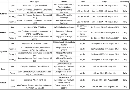
Data  Types Source Unit Range Frequency

Spot WTI  Crude  Oil  Spot  Price  FOB U.S.  Energy  Information  

Administration USD  per  Barrel 2nd  Jan  2009  -­‐    4th  August  2014 Daily Future_1Crude  Oil  Futures,  Continuous  Contract  #1  (CL1)  (Front  Month) Chicago  Mercantile  Exchange USD  per  Barrel 2nd  Jan  2009  -­‐    4th  August  2014 Daily

Future_2Crude  Oil  Futures,  Continuous  Contract  #2   (CL2)

Chicago  Mercantile  

Exchange USD  per  Barrel 2nd  Jan  2009  -­‐    4th  August  2014 Daily Future_3Crude  Oil  Futures,  Continuous  Contract  #3  

(CL3)

Chicago  Mercantile  

Exchange USD  per  Barrel 2nd  Jan  2009  -­‐    4th  August  2014 Daily Spot Iron  Ore,  62%  Fe  CFR  China WSJ  Market  Data  Center cts  per  metric  

tonne 1st  October  2013  -­‐  8th  August  2014 Daily Future_1 Iron  Ore  Futures,  Continuous  Contract  #1  

(FEF1)  (Front  Month)

Singapore  Exchange   Limited

cts  per  metric  

tonne 1st  October  2013  -­‐  8th  August  2014 Daily Future_2 Iron  Ore  Futures,  Continuous  Contract  #2  (FEF2) Singapore  Exchange  Limited cts  per  metric  tonne 1st  October  2013  -­‐  8th  August  2014 Daily

Spot Soybeans,  No.  1  Yellow,  Illinois USDA  via  WSJ  Market  Data  

Center. cts/bu 1st  August  2008  -­‐  5th  August  2014 Daily Future_1 CBOT  Soybeans  Futures,  Continuous  Contract  #1  (S1)  (Front  Month) Chicago  Board  of  Trade  (CBOT) cts/bu 1st  August  2008  -­‐  5th  August  2014 Daily

Future_2 Soybean  Futures,  Continuous  Contract  #2   (S2)

Chicago  Mercantile  

Exchange cts/bu 1st  August  2008  -­‐  5th  August  2014 Daily Future_3 Soybean  Futures,  Continuous  Contract  #3  

(S3)

Chicago  Mercantile  

Exchange cts/bu 1st  August  2008  -­‐  5th  August  2014 Daily

Spot Corn,  No.  2  Yellow,  Central  Illinois

US  Department  of   Agriculture  via  The  Wall  

Street  Journal

cts/bu 4th  Jan  2010  -­‐  17th  July  2014 Daily

Future CBOT  Corn  Futures,  Continuous  Contract  #1  (C1)  (Front  Month) Chicago  Board  of  Trade  (CBOT) cts/bu 4th  Jan  2010  -­‐  17th  July  2014 Daily

Spot Spot  price  Wheat    hard,  KC

US  Department  of   Agriculture  via  The  Wall  

Street  Journal

cts/bu 2nd  Jan  2008  -­‐  19th  August  2014 Daily

Future CBOT  Wheat  Futures,  Continuous  Contract   #1  (W1)  (Front  Month)

Chicago  Board  of  Trade  

(CBOT) cts/bu 2nd  Jan  2008  -­‐  19th  August  2014 Daily Wheat

Crude  Oil

Soybeans Iron  Ore

Corn

The data types, data sources, units, ranges of the data and frequency of the data corresponding to the spot and futures contracts are mentioned in the table below.

(27)

17 WTI crude oil:

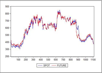
Daily spot rate of West Texas Intermediate (WTI) Crude oil from U.S. Energy Information Administration and its futures contracts published by Chicago Mercantile Exchange for a period from 2nd January 2009 to 4th August 2014 has been analyzed in this study.

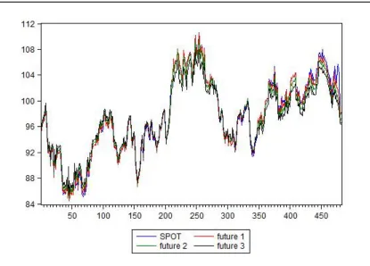
Graph 3. WTI Crude oil spot and futures prices

Source: U.S. Energy Information Administration and Chicago Mercantile Exchange

From the graph, it is observed that the spot and the futures prices move very close to each other through the sample, but around 450 observations till last, there is some deviation between the spot and futures prices. The data shows medium skewness.

Table 2. WTI Crude oil statistics

N  Mean  Std.  Dev.  Skewness  Kurtosis  Jarque-­‐Bera Q(36)

spot 482 4.579 0.064 -­‐0.202 2.239 14.907 467.410

0.001 0.000

future  1 482 4.578 0.062 -­‐0.206 2.299 13.283 467.050

0.001 0.000

future  2 482 4.578 0.057 -­‐0.228 2.414 11.071 465.420

0.004 0.000

future  3 482 4.575 0.052 -­‐0.281 2.510 11.168 462.220

(28)

18 Iron Ore, 62% Fe CFR China:

Daily spot rate of Iron Ore, 62% Fe4 CFR5 China from WSJ Market Data Center and its two futures contracts from Singapore Exchange Limited from 1st October 2013 to 8th August 2014 have been analyzed.

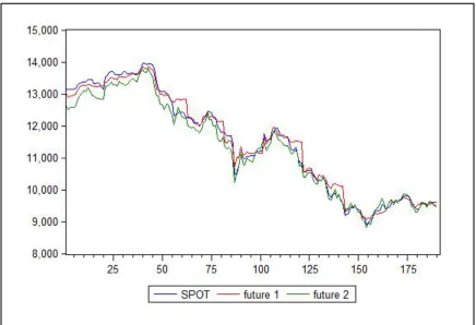
Graph 4. Iron Ore, 62% Fe CFR China spot and futures prices.

Source: WSJ Market Data Center and Singapore Exchange Limited

At the starting of the graph, we can observe huge gaps between the spot and futures prices and throughout the graph there is some difference between the same. This states that the hedging effectiveness would not be very high and there is basis risk involved. Moreover the sample size is also not very high, so, we do not expect a very good result from this. The data shows low skewness.

Table 3. Iron Ore, 62% Fe CFR China statistics

4 Iron

5 Cost and Freight

N  Mean  Std.  Dev.  Skewness  Kurtosis  Jarque-­‐Bera Q(36)

spot 190 9.337 0.140 -­‐0.110 1.595 16.001 188.870

0.000 0.000

future  1 190 9.340 0.136 -­‐0.189 1.615 16.321 188.340

0.000 0.000

future  2 190 9.324 0.131 -­‐0.099 1.648 14.789 188.140

(29)

19 Soybeans, No. 1 Yellow, Illinois:

Daily spot price of Soybeans, No. 1 Yellow, Illinois from USDA via WSJ Market Data Center and its three futures contracts published in Chicago Mercantile Exchange for a period from 1st August 2008 to 5th August 2014 have been considered.

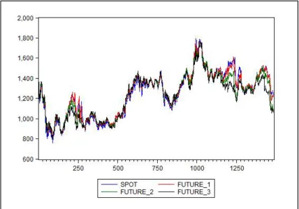
Graph 5. Soybeans, No. 1 Yellow, Illinois spot and futures prices.

Source: USDA via WSJ Market Data Center and Chicago Mercantile Exchange

Though we have very large observations, there is some deviation between the spot and futures prices near observation no. 250 and observation no. 1250. At the end of the graph also we find that futures prices and spot prices are not moving together. This may lead to lower hedging effectiveness. The data shows medium skewness.

Table 4. Soybeans, No. 1 Yellow, Illinois statistics

N  Mean  Std.  Dev.  Skewness  Kurtosis  Jarque-­‐Bera Q(36)

spot 1482 7.107 0.187 -­‐0.345 2.070 82.733 1471.500

0.000 0.000

future  1 1482 7.116 0.179 -­‐0.365 2.039 90.056 1470.500

0.000 0.000

future  2 1482 7.105 0.175 -­‐0.341 1.998 90.703 1470.500

0.000 0.000

future  3 1482 7.093 0.170 -­‐0.305 2.016 82.693 1469.800

(30)

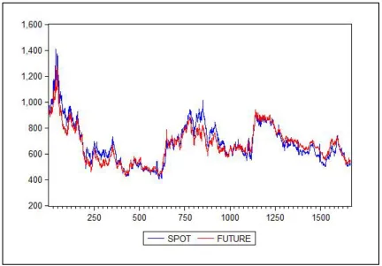
20 Corn, No. 2 Yellow, Central Illinois:

Daily spot price of Corn, No. 2 Yellow, Central Illinois from US Department of Agriculture via The Wall Street Journal and its futures contract from Chicago Board of Trade (CBOT) for a period 4th Jan 2010 to 17th July 2014 has been considered.

Graph 6. Corn, No. 2 Yellow, Central Illinois spot and futures prices.

Source: US Department of Agriculture via the Wall Street Journal and Chicago Board of Trade

We have a large observations for the corn prices and its futures. The spot and futures prices move very close to each other except near observation no. 900 where futures price is much lower than the spot price. The data shows relatively high skewness.

Table 5. Corn, No. 2 Yellow statistics

N  Mean  Std.  Dev.  Skewness  Kurtosis  Jarque-­‐Bera Q(36)

spot 1110 6.323 0.276 -­‐0.610 2.030 112.452 1103.600

0.000 0.000

future 1110 6.335 0.252 -­‐0.504 1.928 100.130 1101.700

(31)

21 Wheat hard, KC:

Daily spot price Wheat hard, KC from US Department of Agriculture via The Wall Street Journal and its futures contract from Chicago Board of Trade (CBOT) for a period 2nd Jan 2008 to 19th August 2014 has been considered.

Graph 7. Wheat hard, KC spot and futures prices

Source: US Department of Agriculture via the Wall Street Journal and Chicago Board of Trade

Though there is large observation, the spot and futures prices do not move very close to each other stating that there may be a basis risk involved which can lead to lower hedging effectiveness. This is the only data showing positive skewness.

Table 6. Wheat hard, KC statistics

N  Mean  Std.  Dev.  Skewness  Kurtosis  Jarque-­‐Bera Q(36)

Spot 1666 6.499 0.223 0.283 2.797 25.069 1639.400

0.000 0.000

Future 1666 6.486 0.200 0.164 2.710 13.316 1642.400

(32)

22

3.4.

Test of Unit Root and Co-integration

The stationarity of natural logarithm of spot and futures prices and their first difference are found out using ADF (Dickey & Fuller, 1981), PP (Phillips & Perron, 1988) and KPSS (Kwiatkowski, Phillips,

Schmidt, & Shin, 1992) test for stationarity. For ADF and PP test, if the magnitude of t-statistics is

greater than the magnitude of test critical value (critical value at 95% for ADF and PP test is -2.88), the series is stationary else not. For KPSS test, if the t-statistics value is lower than the critical value (critical value for the KPSS test is 0.146 for 5%), than the series is stationary else not. The summary of the statistics is given in the following table.

Table 7: Unit root test on price and returns

All the three test statistics confirmed all natural logarithm spot and futures prices in levels are non-stationary and on first difference are non-stationary.

The lag length for the VAR, VECM and VECM-GARCH model is found out using the Akaike information criterion (AIC) (Brooks, 1989) and the Schwarz information criterion (SC) (Schwarz, 1978). In case, the results of both tests do not match, SC is considered as it is stricter and penalize for the degrees of freedom lost.

Table 8: Lag length of spot and futures prices

level ADF PP KPSS RETURN ADF PP KPSS

Spot -­‐2.10 -­‐2.09 1.43 Spot -­‐22.08 -­‐22.09 0.05

Future_1 -­‐2.12 -­‐2.11 1.38 Future_1 -­‐22.43 -­‐22.44 0.05

Future_2 -­‐2.21 -­‐2.24 1.31 Future_2 -­‐22.19 -­‐22.20 0.05

Future_3 -­‐2.38 -­‐2.41 1.25 Future_3 -­‐22.26 -­‐22.27 0.05

Spot -­‐0.65 -­‐0.48 1.57 Spot -­‐11.10 -­‐10.98 0.13

Future_1 -­‐0.43 -­‐0.41 1.57 Future_1 -­‐14.35 -­‐14.34 0.12

Future_2 -­‐0.49 -­‐0.49 1.55 Future_2 -­‐12.68 -­‐12.68 0.11

Spot -­‐1.85 -­‐1.90 3.22 Spot -­‐38.35 -­‐38.35 0.09

Future_1 -­‐2.15 -­‐1.99 3.10 Future_1 -­‐29.48 -­‐40.19 0.09

Future_2 -­‐1.81 -­‐1.87 2.94 Future_2 -­‐37.58 -­‐37.58 0.12

Future_3 -­‐1.87 -­‐1.93 2.69 Future_3 -­‐38.28 -­‐38.28 0.12

Spot -­‐1.28 -­‐1.33 0.98 Spot -­‐31.86 -­‐31.84 0.39

Future -­‐1.41 -­‐1.39 0.88 Future -­‐32.25 -­‐32.24 0.31

Spot -­‐2.63 -­‐2.51 0.42 Spot -­‐43.83 -­‐44.03 0.06

Future -­‐2.77 -­‐2.70 0.37 Future -­‐39.85 -­‐39.90 0.08

Wheat Crude  Oil

Iron  Ore

Soybeans

Corn

Spot-­‐Future  1 Spot-­‐Future  2 Spot-­‐Future  3

Crude  Oil 1 1 1

Iron  Ore 2 1

Soybeans 2 2 1

Corn 1

(33)

23

Hypothesized 0.05 0.05 0.05

No.  of  CE(s)

Critical   Value

Critical   Value

Critical   Value

None   0.102 56.298 20.262 0.000 0.058 32.854 20.262 0.001 0.047 27.127 20.262 0.005

At  most  1 0.009 4.506 9.165 0.342 0.009 4.426 9.165 0.352 0.008 3.870 9.165 0.432

None 0.140 28.640 15.495 0.000 0.191 40.006 15.495 0.000

At  most  1 0.002 0.414 3.841 0.520 0.001 0.206 3.841 0.650

None 0.041 65.454 15.495 0.000 0.006 12.553 15.495 0.132 0.003 8.246 15.495 0.439

At  most  1 0.002 3.168 3.841 0.075 0.002 3.222 3.841 0.073 0.002 3.373 3.841 0.066

None 0.018 21.203 15.495 0.006

At  most  1 0.001 1.502 3.841 0.220

None 0.010 24.125 20.262 0.014

At  most  1 0.005 7.776 9.165 0.091

Trace  Statistic P-­‐value

Spot-­‐Future  1 Spot-­‐Future  2 Spot-­‐Future  3

Eigenvalue Trace  Statistic P-­‐value Eigenvalue Trace  Statistic P-­‐value Eigenvalue

Wheat Crude  Oil

Iron  Ore

Soybeans

Corn

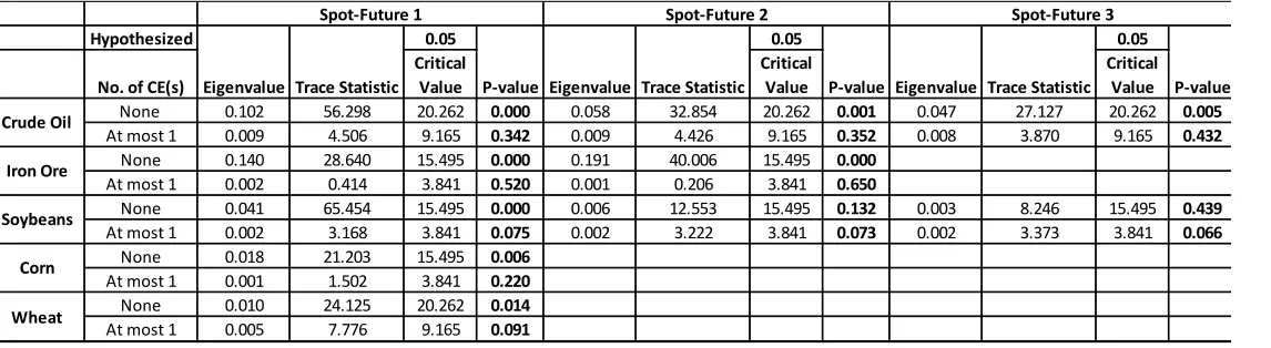
To find if there is co-integration between the spot and futures prices, Johansen’s (1991) maximum likelihood method is used. The result of the co-integration in presented in the following table. Table 9: Johansen co-integration test of spot and futures prices

From the above table, we find that, all spot and futures prices are co-integrated, and hence there exist a long term relationship between them except the following:

a) Spot and future 1 of crude oil b) Spot and future 2 of crude oil c) Spot and future of wheat.

From graph 3, two major cycle of spot and futures prices of the crude oil can be observed. The price has varied from as low as 84 USD/barrel to as high as 110 USD/barrel. Moreover, at the end of the observations, we find that, the futures prices are not moving close to the spot prices which also leads to no long run relationship between them.

(34)

24

Corn Wheat

Future_1 Future_2 Future_3 Future_1 Future_2 Future_1 Future_2 Future_3 Future Future

α 3.16E-­‐05 5.52E-­‐05 7.44E-­‐05 -­‐7.77E-­‐04 -­‐7.22E-­‐04 5.66E-­‐06 8.04E-­‐05 9.51E-­‐05 4.80E-­‐05 -­‐6.76E-­‐05

β 0.994 1.012 1.032 0.563 0.635 0.871 0.927 0.933 0.781 0.890 R2 95.55% 93.94% 91.90% 44.84% 54.69% 75.25% 77.73% 76.02% 69.47% 57.53%

Soybeans

Crude  Oil Iron  Ore

Corn Wheat Future_1 Future_2 Future_3 Future_1 Future_2 Future_1 Future_2 Future_3 Future Future

β 0.980 0.996 1.022 0.579 0.643 0.930 0.953 0.942 0.980 0.859

R2 94.49% 93.23% 91.31% 41.20% 54.65% 73.38% 76.98% 75.62% 64.80% 53.77%

Crude  Oil Iron  Ore Soybeans

4.

Empirical Results

The hedge ratio and hedging effectiveness of the commodity futures (crude oil, iron ore, soybeans, corn and wheat) is estimated through four models (OLS, VAR, VECM and bivariate GARCH) and compared with the naive hedge ratio as described earlier. The time varying hedge ratio using VAR / VECM – GARCH method is also calculated. The hedge ratio and hedging effectiveness using both in-sample and out-of-in-sample method is calculated in this study.

4.1.

In-sample Results

4.1.1.

OLS and OLS-GARCH Estimations

Equation 6 and Equation 7 is used to calculate the following hedge ratio and hedging effectiveness using OLS and OLS-GARCH model respectively. The co-efficient of the independent variable, that is, the slope off the equation denotes the optimal hedge ratio (β) of the futures and the R2 of the equation denotes the hedging effectiveness.

Table 10: OLS regression model estimations

Table 11: OLS-GARCH model estimations

The hedge ratio estimation by both methods provide approximately 90% variance reduction for crude oil, 75% variance reduction for soybeans futures and about 70% variance reduction for corn and wheat. Iron ore futures have the lowest hedging effectiveness among all, that is, 45% for near month futures contract and 55% for next near month futures contract (for OLS model). One of the reasons for low hedging effectiveness for iron ore futures is the low sample size. We also observe that the hedging effectiveness decreases as we move from the near month to distance futures for crude oil, but the same pattern is not found for iron ore and soybeans futures.

4.1.2.

VAR Estimations

(35)

25

Corn Wheat

Future_1 Future_2 Future_3 Future_1 Future_2 Future_1 Future_2 Future_3 Future Future β1 1.12E-­‐01 1.22E-­‐01 1.30E-­‐01 1.51E-­‐01 -­‐1.76E-­‐01 -­‐1.75E-­‐01 -­‐1.34E-­‐01 -­‐1.17E-­‐01 -­‐1.66E-­‐02 -­‐2.59E-­‐01

β2 -­‐1.16E-­‐01 -­‐1.08E-­‐01 8.84E-­‐03 -­‐1.30E-­‐01

β3 -­‐3.22E-­‐02

γ1 -­‐1.35E-­‐01 -­‐1.50E-­‐01 -­‐1.66E-­‐01 7.01E-­‐02 4.34E-­‐01 1.86E-­‐01 1.47E-­‐01 1.32E-­‐01 6.41E-­‐02 2.06E-­‐01

γ2 1.07E-­‐01 9.61E-­‐02 -­‐3.49E-­‐02 1.37E-­‐01

γ3 6.87E-­‐02

α 5.89E-­‐05 5.51E-­‐05 5.16E-­‐05 -­‐1.35E-­‐03 -­‐1.32E-­‐03 -­‐1.06E-­‐05 -­‐4.07E-­‐06 -­‐1.30E-­‐05 -­‐2.08E-­‐05 -­‐3.53E-­‐04

R2 1.23E-­‐03 1.65E-­‐03 2.33E-­‐03 5.23E-­‐02 1.55E-­‐01 9.93E-­‐03 5.35E-­‐03 3.83E-­‐03 3.13E-­‐03 3.17E-­‐02 Spot  Prices

Crude  Oil Iron  Ore Soybeans

Corn Wheat

Future_1 Future_2 Future_3 Future_1 Future_2 Future_1 Future_2 Future_3 Future Future

β1 -­‐2.71E-­‐01 -­‐2.23E-­‐01 -2.33E-01 -­‐5.09E-­‐02 2.23E-­‐01 -­‐2.51E-­‐02 -­‐2.51E-­‐02 -­‐2.15E-­‐02 -­‐7.51E-­‐02 -5.86E-02 β2 -­‐5.33E-­‐02 1.56E-­‐02 -­‐3.43E-­‐02 -5.15E-02

β3 -4.40E-02

γ1 2.40E-­‐01 1.96E-­‐01 2.01E-01 -­‐2.14E-­‐02 -­‐2.56E-­‐01 7.00E-­‐02 4.97E-­‐02 2.91E-­‐02 1.32E-­‐01 3.14E-02

γ2 1.36E-­‐01 -­‐1.90E-­‐02 2.60E-­‐02 4.75E-02

γ3 2.33E-02

α 6.12E-­‐05 2.81E-­‐05 4.01E-06 -­‐1.61E-­‐03 -­‐1.56E-­‐03 -­‐2.11E-­‐05 -­‐1.08E-­‐04 -­‐1.33E-­‐04 -­‐9.88E-­‐05 -3.15E-04 R2 4.36E-­‐03 3.43E-­‐03 4.76E-­‐03 1.33E-­‐02 2.55E-­‐02 2.80E-­‐03 1.23E-­‐03 2.70E-­‐04 5.40E-­‐03 3.05E-­‐03

Future  Prices

Crude  Oil Iron  Ore Soybeans

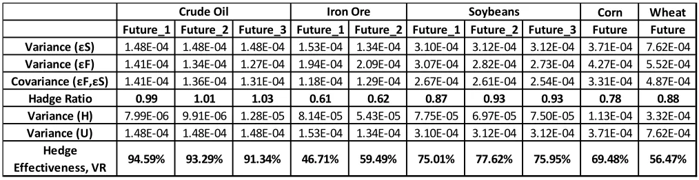
Corn Wheat Future_1 Future_2 Future_3 Future_1 Future_2 Future_1 Future_2 Future_3 Future Future Variance  (εS) 1.48E-­‐04 1.48E-­‐04 1.48E-­‐04 1.53E-­‐04 1.34E-­‐04 3.10E-­‐04 3.12E-­‐04 3.12E-­‐04 3.71E-­‐04 7.62E-­‐04

Variance  (εF) 1.41E-­‐04 1.34E-­‐04 1.27E-­‐04 1.94E-­‐04 2.09E-­‐04 3.07E-­‐04 2.82E-­‐04 2.73E-­‐04 4.27E-­‐04 5.52E-­‐04

Covariance  (εF,εS) 1.41E-­‐04 1.36E-­‐04 1.31E-­‐04 1.18E-­‐04 1.29E-­‐04 2.67E-­‐04 2.61E-­‐04 2.54E-­‐04 3.31E-­‐04 4.87E-­‐04

Hadge  Ratio 0.99 1.01 1.03 0.61 0.62 0.87 0.93 0.93 0.78 0.88

Variance  (H) 7.99E-­‐06 9.91E-­‐06 1.28E-­‐05 8.14E-­‐05 5.43E-­‐05 7.75E-­‐05 6.97E-­‐05 7.50E-­‐05 1.13E-­‐04 3.32E-­‐04

Variance  (U) 1.48E-­‐04 1.48E-­‐04 1.48E-­‐04 1.53E-­‐04 1.34E-­‐04 3.10E-­‐04 3.12E-­‐04 3.12E-­‐04 3.71E-­‐04 7.62E-­‐04

Hedge  

Effectiveness,  VR 94.59% 93.29% 91.34% 46.71% 59.49% 75.01% 77.62% 75.95% 69.48% 56.47%

Crude  Oil Iron  Ore Soybeans

equations are presented in the Table 12. The optimal hedge ratio and the hedging effectiveness are also presented in Table 13.

Table 12: Estimations of VAR model

a) Spot prices

b) Futures prices

(36)

26

Crude  Oil Corn Wheat

Future_1 Future_2 Future_3 Future_1 Future_2 Future_1 Future_2 Future_3 Future Future

β 1.04E-­‐01 -­‐1.97E-­‐02 -­‐2.86E-­‐01 -­‐1.84E-­‐02 -­‐1.31E-­‐02 -­‐5.69E-­‐03 -­‐2.60E-­‐02

β1 7.59E-­‐02 1.61E-­‐01 -­‐1.26E-­‐01 -­‐1.64E-­‐01 -­‐1.26E-­‐01 -­‐1.14E-­‐01 -­‐8.36E-­‐03

β2 -­‐1.03E-­‐01 -­‐1.00E-­‐01 1.52E-­‐02

γ -­‐1.33E-­‐01 2.02E-­‐02 3.07E-­‐01 1.93E-­‐02 1.41E-­‐02 6.43E-­‐03 2.87E-­‐02

γ1 -­‐9.72E-­‐02 6.16E-­‐02 2.72E-­‐01 1.74E-­‐01 1.37E-­‐01 1.28E-­‐01 4.97E-­‐02

γ2 9.92E-­‐02 8.79E-­‐02 -­‐4.23E-­‐02

α 1.30E-01 -­‐5.92E-­‐03 -­‐1.99E-­‐01 -­‐6.72E-­‐03 -­‐7.16E-­‐03 -­‐5.15E-­‐03 -­‐1.76E-­‐02

R2 8.90E-­‐03 5.27E-­‐02 2.06E-­‐01 1.03E-­‐02 6.18E-­‐03 4.20E-­‐03 7.65E-­‐03

Spot  Prices

Iron  Ore Soybeans

Corn Wheat

Future_1 Future_2 Future_3 Future_1 Future_2 Future_1 Future_2 Future_3 Future Future

β -2.07E-01 -­‐2.75E-­‐01 -­‐6.60E-­‐02 -­‐8.68E-­‐02 -­‐4.49E-­‐03 -­‐3.03E-­‐03 -­‐3.20E-­‐03

β1 -­‐1.26E-­‐01 6.51E-­‐02 2.58E-­‐01 2.50E-­‐02 -­‐2.21E-­‐02 -­‐1.97E-­‐02 -­‐7.35E-­‐02

β2 5.43E-­‐02 5.24E-­‐02 -­‐3.20E-­‐02

γ 1.63E-01 2.69E-­‐01 6.13E-­‐02 8.27E-­‐02 4.17E-­‐03 2.69E-­‐03 2.90E-­‐03

γ1 1.16E-­‐01 -­‐1.52E-­‐01 -­‐2.66E-­‐01 2.14E-­‐02 4.70E-­‐02 2.77E-­‐02 1.31E-­‐01

γ2 -­‐3.62E-­‐02 -­‐5.25E-­‐02 2.40E-­‐02

α 2.03E-01 6.09E-­‐02 4.09E-­‐02 3.02E-­‐02 2.17E-­‐03 1.86E-­‐03

R2 2.34E-­‐02 7.91E-­‐02 2.73E-­‐02 9.97E-­‐03 1.32E-­‐03 3.64E-­‐04 5.44E-­‐03

Iron  Ore Soybeans

Future  Prices Crude  Oil

Generally the hedge ratio calculated by VAR model are higher and performs better than OLS model in reducing the variance. The hedge ratio estimated through VAR model changed from 0.56 and 0.61 (OLS estimation) to 0.61 and 0.62 (VAR estimation) leading to increased hedging effectiveness from 45% to 47% and from 55% to 60% for iron ore future 1 and iron ore future 2 respectively. In other futures contracts, there is not much increase in the hedging effectiveness stating that, for the aforementioned commodities, OLS and VAR models perform almost the same.

4.1.3.

VECM Estimations

Vector error correction model can only be executed for the model which has long run relationship between the spot and futures prices. This model also has the same approach as that of the VAR model where the estimated errors help in calculation of the hedge ratio and the hedging effectiveness. Table 14 shows the parameters of the VECM model. The optimal hedge ratio and the hedging effectiveness is shown in Table 15.

Table 14: Estimations of VECM model

a) Spot prices

(37)

27 Corn Wheat

Future_1 Future_2 Future_3 Future_1 Future_2 Future_1 Future_2 Future_3 Future Future Variance  (εS) 1.47E-­‐04 1.54E-­‐04 1.27E-­‐04 3.10E-­‐04 3.11E-­‐04 3.12E-­‐04 3.69E-­‐04

Variance  (εF) 1.25E-­‐04 1.82E-­‐04 2.10E-­‐04 3.05E-­‐04 2.82E-­‐04 2.73E-­‐04 4.27E-­‐04 Covariance  (εF,εS) 1.30E-­‐04 1.19E-­‐04 1.32E-­‐04 2.68E-­‐04 2.61E-­‐04 2.55E-­‐04 3.32E-­‐04

Hadge  Ratio 1.037 0.655 0.627 0.878 0.927 0.931 0.777

Variance  (H) 1.24E-­‐05 7.55E-­‐05 4.43E-­‐05 7.49E-­‐05 6.93E-­‐05 7.48E-­‐05 1.11E-­‐04 Variance  (U) 1.47E-­‐04 1.54E-­‐04 1.27E-­‐04 3.10E-­‐04 3.11E-­‐04 3.12E-­‐04 3.69E-­‐04

Hedge  

Effectiveness,  E 91.54% 50.88% 65.08% 75.86% 77.74% 76.02% 69.88%

Crude  Oil Iron  Ore Soybeans

Corn Wheat

Future_1 Future_2 Future_3 Future_1 Future_2 Future_1 Future_2 Future_3 Future Future Variance  (εS) 1.47E-­‐04 1.47E-­‐04 1.48E-­‐04 1.52E-­‐04 1.25E-­‐04 3.10E-­‐04 3.10E-­‐04 3.11E-­‐04 3.71E-­‐04 7.69E-­‐04 Variance  (εF) 1.40E-­‐04 1.34E-­‐04 1.25E-­‐04 1.78E-­‐04 2.06E-­‐04 3.06E-­‐04 2.81E-­‐04 2.73E-­‐04 4.36E-­‐04 5.55E-­‐04 Covariance  (εF,εS) 1.40E-­‐04 1.36E-­‐04 1.30E-­‐04 1.17E-­‐04 1.29E-­‐04 2.68E-­‐04 2.60E-­‐04 2.54E-­‐04 3.36E-­‐04 4.90E-­‐04

Hadge  Ratio 0.994 1.013 1.040 0.656 0.627 0.875 0.926 0.930 0.771 0.884

Variance  (H) 8.05E-­‐06 9.93E-­‐06 1.27E-­‐05 7.50E-­‐05 4.35E-­‐05 7.58E-­‐05 6.94E-­‐05 7.48E-­‐05 1.12E-­‐04 3.36E-­‐04 Variance  (U) 1.47E-­‐04 1.47E-­‐04 1.48E-­‐04 1.52E-­‐04 1.25E-­‐04 3.10E-­‐04 3.10E-­‐04 3.11E-­‐04 3.71E-­‐04 7.69E-­‐04

Hedge  

Effectiveness,  E 94.52% 93.26% 91.43% 50.57% 65.08% 75.57% 77.64% 75.96% 69.91% 56.28%

Crude  Oil Iron  Ore Soybeans Table 15. Estimation of hedge ratio and hedging effectiveness for VECM model.

Though the time varying conditional covariance structure of spot and futures prices is not considered in VECM model, still it is considered as the best model for capturing the constant hedge ratio and hedging effectiveness as it takes into account the long term co-integration between the spot and futures prices. As we can see from the table, parameters for crude oil (future 1 and future 2) and wheat are not mentioned in the table as they could not satisfy co-integration in Johansen’s test.

4.1.4.

Bivariate-GARCH Estimations

Bivariate – GRACH model is used to capture the time varying volatility to the hedge ratio and also to incorporate the non-linearity in the mean equation. The model is developed from VECM model for the variables which show a long run relationship between futures and spot prices and from VAR model for the variables which don’t satisfy the same condition. The “ARCH effect” of the error terms found from the VAR and VECM models are analyzed. VAR / VECM models with bivariate diagonal GARCH (1, 1) are used. The time varying hedge ratio and hedging effectiveness for the commodities are estimated using GARCH (1, 1) parameters obtained from Equation 12.

(38)

28

Corn Wheat

Future_1 Future_2 Future_3 Future_1 Future_2 Future_1 Future_2 Future_3 Future Future

Variance  (εS) 1.39E-­‐04 1.38E-­‐04 1.37E-­‐04 1.53E-­‐04 1.56E-­‐04 3.15E-­‐04 3.18E-­‐04 3.19E-­‐04 3.64E-­‐04 7.73E-­‐04 Variance  (εF) 1.41E-­‐04 1.34E-­‐04 1.27E-­‐04 1.90E-­‐04 2.10E-­‐04 3.09E-­‐04 2.83E-­‐04 2.75E-­‐04 4.27E-­‐04 5.52E-­‐04 Covariance  (εF,εS) 1.39E-­‐04 1.34E-­‐04 1.29E-­‐04 1.11E-­‐04 1.36E-­‐04 2.71E-­‐04 2.67E-­‐04 2.63E-­‐04 3.29E-­‐04 4.82E-­‐04

Hadge  Ratio 0.98 1.00 1.02 0.58 0.65 0.88 0.94 0.96 0.77 0.87

Variance  (H) 2.60E-­‐06 3.94E-­‐06 6.11E-­‐06 8.82E-­‐05 6.83E-­‐05 7.70E-­‐05 6.56E-­‐05 6.70E-­‐05 1.10E-­‐04 3.52E-­‐04 Variance  (U) 1.39E-­‐04 1.38E-­‐04 1.37E-­‐04 1.53E-­‐04 1.56E-­‐04 3.15E-­‐04 3.18E-­‐04 3.19E-­‐04 3.64E-­‐04 7.73E-­‐04

Hedge  

Effectiveness,  VR 98.13% 97.14% 95.55% 42.25% 56.22% 75.54% 79.35% 78.99% 69.77% 54.49%

Crude  Oil Iron  Ore Soybeans

Corn Wheat Future_1 Future_2 Future_3 Future_1 Future_2 Future_1 Future_2 Future_3 Future Future Variance  (εS) 1.39E-­‐04 1.37E-­‐04 1.37E-­‐04 1.53E-­‐04 1.56E-­‐04 3.16E-­‐04 3.18E-­‐04 3.19E-­‐04 3.70E-­‐04 7.73E-­‐04 Variance  (εF) 1.41E-­‐04 1.34E-­‐04 1.27E-­‐04 1.90E-­‐04 2.10E-­‐04 3.09E-­‐04 2.83E-­‐04 2.75E-­‐04 4.27E-­‐04 5.52E-­‐04 Covariance  (εF,εS) 1.38E-­‐04 1.34E-­‐04 1.29E-­‐04 1.11E-­‐04 1.36E-­‐04 2.71E-­‐04 2.67E-­‐04 2.63E-­‐04 3.33E-­‐04 4.82E-­‐04

Hadge  Ratio 0.98 1.00 1.02 0.58 0.65 0.88 0.95 0.96 0.78 0.87 Variance  (H) 2.60E-­‐06 3.94E-­‐06 6.10E-­‐06 8.82E-­‐05 6.83E-­‐05 7.70E-­‐05 6.56E-­‐05 6.70E-­‐05 1.11E-­‐04 3.52E-­‐04 Variance  (U) 1.39E-­‐04 1.37E-­‐04 1.37E-­‐04 1.53E-­‐04 1.56E-­‐04 3.16E-­‐04 3.18E-­‐04 3.19E-­‐04 3.70E-­‐04 7.73E-­‐04

Hedge  

Effectiveness,  VR 98.13% 97.13% 95.54% 42.28% 56.24% 75.61% 79.38% 79.02% 70.08% 54.46%

Crude  Oil Iron  Ore Soybeans

4.2.

Out-of-sample Empirical Results

Hedgers should use the results of out-of-sample models for hedging effectiveness as it is more concerned about the futures performance (Brooks & Chong, 2001). To calculate that, the initial position of the observations combined with the out-of-sample forecast estimation is used. Data of a period of 7th April 2014 to 4th August 2014 is used for out of sample analysis for crude

Figure

Table 1. Data Information
Table 2. WTI Crude oil statistics
Table 3. Iron Ore, 62% Fe CFR China statistics
Table 4. Soybeans, No. 1 Yellow, Illinois statistics
+7

References

Related documents