VAPOR COMPRESSION SYSTEMS
by Travis D. Pruitt
A thesis
submitted in partial fulfillment of the requirements for the degree of Master of Science in Mechanical Engineering
Boise State University
DEFENSE COMMITTEE AND FINAL READING APPROVALS
of the thesis submitted by
Travis D. Pruitt
Thesis Title: Parameter Estimation and Dynamic State Observer Design for Vapor Compression Systems
Date of Final Oral Examination: 7 June 2019
The following individuals read and discussed the thesis submitted by student Travis D. Pruitt, and they evaluated his presentation and response to questions during the final oral examination. They found that the student passed the final oral examination.
John F. Gardner, Ph.D. Chair, Supervisory Committee Donald Plumlee, Ph.D. Member, Supervisory Committee Ralph S. Budwig, Ph.D. Member, Supervisory Committee
iv
I would like to take a moment to thank those who’s mentorship and guidance has been greatly appreciated throughout, not only this thesis, but my academic career
altogether. First, Dr. John Gardner. Not only has Dr. Gardner become a good friend, but the experience I’ve gained working with him on various projects over the past several years has been invaluable. Thank you for your continued support and patients while I finished this thesis while working full-time.
I would also like to thank Dr. Plumlee and Dr. Budwig for their insight and
direction that helped me to bring this thesis to completion. I was fortunate enough to have had the opportunity to attend classes taught by each of you, and truly appreciate the impact each of you had on both my academic and professional careers.
v
Between cooling our house, our workplace, and keeping our food cold both in home and commercially (among other uses), the vapor compression cycle (VCC) is a common method for removing heat from various environments and it accounts for a significant amount of the energy used throughout the world. Therefore, with an ever-growing demand for more efficient processes and reduced energy consumption,
improving the ability to accurately model, predict the performance of, and control VCC systems is beneficial to society as whole.
While there is much information available regarding the performance for some of the components found in VCC systems, much of the challenge associated with modelling the VCC lies within the complex behavior of the heat exchangers found within the system. Over the years, lumped parameter models have been developed for the VCC. However, many of these rely on simplified geometry (mainly a bare tube assumption), and neglect to capture the effect of the fins found throughout those heat exchangers.
This thesis builds upon approaches used in the past by identifying effective heat transfer coefficients that capture this effect. Using this approach, a 2-ton residential air-conditioning unit was modelled, which was able to predict the heat removed by the VCC system within ±4% error when compared to published performance data from the
vi
ACKNOWLEDGEMENTS ... iv
ABSTRACT ...v
LIST OF TABLES ... viii
LIST OF FIGURES ... ix
CHAPTER ONE: INTRODUCTION ...1
CHAPTER TWO: LITERATURE REVIEW ...8
Condenser Dynamics ...10
Evaporator Dynamics...12
Compressor Thermodynamics ...13
Thermodynamics of the Expansion Valve ...14
Lumped Parameter Dynamic Model & State Equations ...15
Observer Design...18
Thesis Contributions ...20
CHAPTER THREE: DYNAMIC MODEL PARAMETER IDENTIFICATION ...21
Parameter Identification Based on System Data: ...21
CHAPTER FOUR: DYNAMIC MODEL AND CALIBRATION ...26
Model Development...26
Parameter Identification for Effective Fin Coefficients (UA’) ...27
vii
Measured States for the Evaporator ...34
Nonlinear Observer Implementation ...34
CHAPTER SIX: CONCLUSION ...41
Future Work ...42
REFERENCES ...44
APPENDIX A ...46
Example Manufacturer Data Set ...46
APPENDIX B ...48
Compressor Model ...48
APPENDIX C ...50
viii
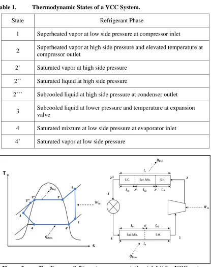
Table 1. Thermodynamic States of a VCC System. ... 4
Table 2. Heat Removed by Model Compared to Literature. ... 28
Table 3. Example Effective Coefficients Sets ... 28
Table 4. 𝑼𝑼𝑼𝑼𝑼𝑼𝑼𝑼′ Coefficients ... 30
Table 5. Dynamic Model Results Outdoor Air Temp. Range 65 °F – 85 °F ... 31
Table 6. Dynamic Model Results Outdoor Air Temp. Range 95 °F – 115 °F ... 31
Table 7. Nonlinear State Observer Gain Values ... 35
ix
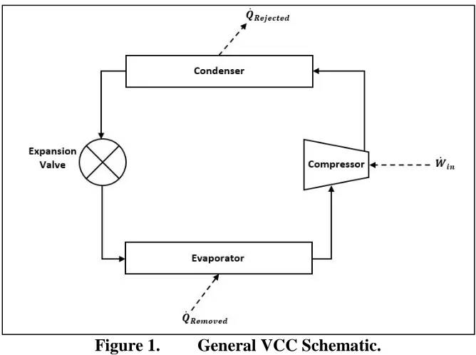
Figure 1. General VCC Schematic. ... 2
Figure 2. Condenser Tubing and Portion of Fins on Residential HVAC unit. ... 3
Figure 3. T-s diagram (left), system representation (right) for VCC system. ... 4
Figure 4. Goodman Residential Air Conditioning Unit. ... 6
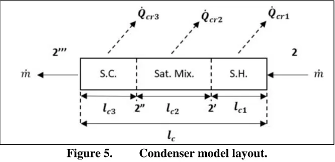
Figure 5. Condenser model layout. ... 10
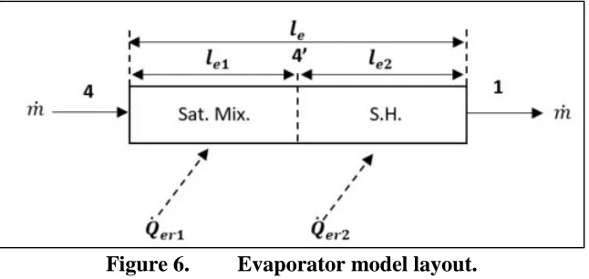
Figure 6. Evaporator model layout. ... 12
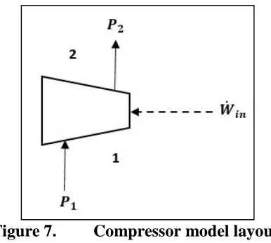
Figure 7. Compressor model layout. ... 13
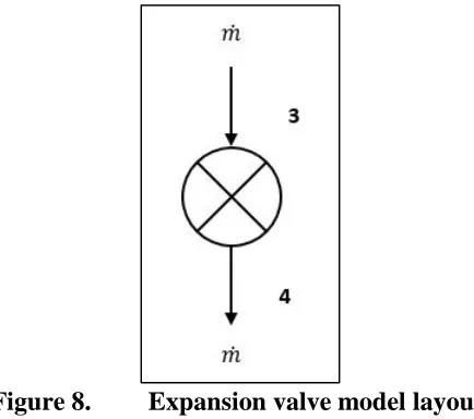
Figure 8. Expansion valve model layout. ... 14
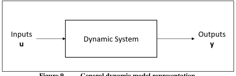
Figure 9. General dynamic model representation. ... 16
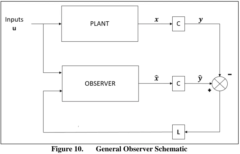
Figure 10. General Observer Schematic ... 19
Figure 11. Simulink Model of VCC System. ... 27
Figure 12. Effective Condenser Fin Coefficient. ... 29
Figure 13. Effective Evaporator Fin Coefficient. ... 29
Figure 14. Existing pressure ports on 2-ton Goodman unit. ... 33
Figure 15. Four measurement observer model. ... 34
Figure 16. Inside observer block of the four-measurement observer. ... 35
x
Figure 21. 2-Measurement observer convergence time comparison. ... 39 Figure 22. Sample Manufacturer's Performance Data. ... 47 Figure 23. Convergence plots for measured and estimated states of the
CHAPTER ONE: INTRODUCTION
The vapor compression cycle (VCC) is the most common refrigeration cycle used to remove heat from a wide variety of processes. (Cengel & Boles, 2015) From large scale commercial cooling to single residence HVAC and refrigeration, the VCC accounts for a significant amount of the energy used throughout the world. However, even with its frequent use, the ability to monitor real time performance or apply advanced control algorithms in VCC systems is still very limited. With an ever-growing demand for more efficient processes and reduced energy consumption, improving our collective ability to model, predict the performance of, and control VCC systems could benefit society as a whole.
Figure 1. General VCC Schematic.
As shown, the tubing throughout each heat exchanger is surrounded by fins. However, previous modelling attempts (discussed further below), frequently utilize equations describing a bare tube to estimate the heat transfer between the refrigerant and its surroundings. While this assumption simplifies the parameter identification, it doesn’t accurately capture what is occurring and ignores a significant component of the system.
In addition, the refrigerant flowing through each heat exchanger experiences various phase changes depending on its thermodynamic state and location throughout the cycle. A summary of the thermodynamic states throughout the VCC can be outlined as shown in Table 1 (which refers to Figure 3) below:
Table 1. Thermodynamic States of a VCC System.
State Refrigerant Phase
1 Superheated vapor at low side pressure at compressor inlet
2 Superheated vapor at high side pressure and elevated temperature at compressor outlet
2’ Saturated vapor at high side pressure 2’’ Saturated liquid at high side pressure
2’’’ Subcooled liquid at high side pressure at condenser outlet 3 Subcooled liquid at lower pressure and temperature at expansion
valve
4 Saturated mixture at low side pressure at evaporator inlet 4’ Saturated vapor at low side pressure
Figure 3. T-s diagram (left), system representation (right) for VCC system.
To model this cycle in such a way to be useful when either controlling or
This approach breaks each heat exchanger into various segments or control volumes to be evaluated.
One version of this approach is to break the heat exchanger into many fixed length segments. However, this increases the number of control volumes or segments to be considered. Another version, the moving boundary method, uses a minimum number of control volumes (segments), the length of which vary as operating conditions change, capturing what occurs in the actual device (Gardner & Luthman, 2016). The benefit of using a lumped parameter approach to represent the VCC system is its ability to reduce the dependence on spatial coordinates and utilize ordinary differential equations, rather than rely on a much higher number of zones with fixed lengths (like an FEA approach). As mentioned in (Matko, Geiger, & Werner, 2001) this method is also useful for
controller/observer design.
research could be used to provide better approximations for design purposes or develop the tools necessary to monitor real-time performance in physical systems used throughout the commercial and residential industries.
For this thesis, a 2-ton Goodman residential HVAC unit utilizing the refrigerant R410a (Model: GSX130241DA, shown in Figure 4) was simulated due to its readily accessible manufacturer’s data on cooling performance (Goodman Air Conditioning & Heating), as well as its intended use in future experimental validation. As such, relevant data about the system including: the high and low operating pressures, refrigerant used, heat removed from the system, and power consumed for certain operating points were readily available1.
Figure 4. Goodman Residential Air Conditioning Unit.
In chapter 2, relevant papers referenced throughout this thesis are reviewed in order to outline the background used to develop the necessary heat transfer coefficients. Chapter 3 identifies the parameters necessary to build both the dynamic VCC model and the nonlinear observer. Chapter 4 outlines the calibration process for the heat transfer
CHAPTER TWO: LITERATURE REVIEW
Much of the research performed in modelling VCC systems to date is primarily focused on steady-state and empirical methods. However, an increasing number of researchers have been turning their focus toward more dynamic models and simulations (Luthman, 2016).
Starting with first principles, He developed a lumped parameter model using the moving boundary approach (He, 1996). Through extensive experimental testing, this model was shown to be relatively effective at capturing the main dynamic characteristics of a VCC. Most recently, research was conducted that led to the development of a quasi-steady state model to identify the heat transfer characteristics of both the evaporator and condenser of a VCC from performance data provided by the manufacturer (Luthman, 2016). This approach utilizes the moving boundary method used by Li (2009) and various others including McKinley & Alleyne (2008), Frink (2005), and Rasmussen (2005), all of whom rely heavily on the work presented in He (1996). As such, the model presented in He (1996) is the backbone for the research presented below and is summarized in more detail to follow.
While some of the more recent research has incorporated the fins into the model of VCC systems, this was done through testing physical systems in a lab setting.
the effect of the fins throughout each heat exchanger. Utilizing these effective coefficients, could potentially eliminate the need for obtaining and testing a physical system prior to predicting the response or performance of a specific unit.
However, the steady state equations proved to be numerically ill conditioned and did not converge well. As such, much of the work presented by Luthman (2016) and Gardner & Luthman (2016) is re-evaluated throughout this thesis prior to expanding on the lumped parameter model provided by He (1996), and the implementation of a nonlinear observer to monitor performance of the system.
As described in Luthman (2016) and He (1996), a thermodynamic analysis of the heat exchangers used throughout a VCC system can be used to mathematically define the heat transfer phenomenon occurring in each. To do so, the following assumptions were made:
• The heat exchangers can be modelled as a single long tube. • The pressure drop across each heat exchanger is negligible.
• The ambient air temperatures surrounding the evaporator and condenser are uniform.
• Due to the relatively high thermal conductivity of the tube wall (usually copper or aluminum) relative to the surrounding media, the temperature of the tube wall is assumed to be uniform in the radial direction.
Condenser Dynamics
Figure 5. Condenser model layout.
Each region within the condenser can be identified and defined by the phase of the refrigerant within (superheated vapor, saturated mixture, and subcooled liquid). Starting within the superheated region, defined between states 2 and 2’ in Figure 5 above, a comparison of the energy balance and heat loss within results in Equation (1) (He, 1996).
𝑚𝑚̇𝑐𝑐𝑐𝑐(ℎ2− ℎ2′) +𝛼𝛼𝑐𝑐𝑐𝑐1𝜋𝜋𝐷𝐷𝑐𝑐𝑐𝑐𝑙𝑙𝑐𝑐1(𝑇𝑇𝑐𝑐𝑐𝑐1− 𝑇𝑇𝑐𝑐𝑐𝑐1) = 0 (1) Where:
𝑚𝑚̇𝑐𝑐𝑐𝑐 – Is the mass flowrate into the condenser [kg/s].
ℎ2 – The specific enthalpy at state 2 [kJ/kg].
ℎ2′ – The specific enthalpy at state 2’ [kJ/kg].
𝛼𝛼𝑐𝑐𝑐𝑐1 – The internal convection heat transfer coefficient of the refrigerant in region
1 [W/m2K].
𝐷𝐷𝑐𝑐𝑐𝑐 – The inner diameter of the condenser tubing [m].
𝑙𝑙𝑐𝑐1 – The instantaneous length of region 1 [m].
𝑇𝑇𝑐𝑐𝑐𝑐1 – The bulk refrigerant temperature in region 1 [K].
The energy balance of the heat transfer external to the tube leads to the following equation on a per unit length basis. It is important to note that this equation assumes the heat exchanger is made up of a bare tube, rather than the actual fins that are in place.
𝛼𝛼𝑐𝑐𝑐𝑐1𝜋𝜋𝐷𝐷𝑐𝑐𝑐𝑐(𝑇𝑇𝑐𝑐𝑐𝑐1− 𝑇𝑇𝑐𝑐𝑐𝑐1) +𝛼𝛼𝑐𝑐𝑐𝑐1𝜋𝜋𝐷𝐷𝑐𝑐𝑐𝑐(𝑇𝑇𝑐𝑐𝑜𝑜− 𝑇𝑇𝑐𝑐𝑐𝑐1) = 0 (2)
Where:
𝛼𝛼𝑐𝑐𝑐𝑐1 – Is the convective heat transfer coefficient for the tube in region 1
[W/m2K].
𝐷𝐷𝑐𝑐𝑐𝑐 – The outer diameter of the condenser tubing [m].
𝑇𝑇𝑐𝑐𝑜𝑜 – The free stream temperature of the outdoor air surrounding the condenser
[K].
Using the same approach, the following equations can be defined for condenser region 2 (between states 2’ and 2’’) and region 3 (between states 2’’ and 2’’’) as outlined in Equations (3) – (6):
𝑚𝑚̇𝑐𝑐𝑐𝑐(ℎ2′ − ℎ2′′) +𝛼𝛼𝑐𝑐𝑐𝑐2𝜋𝜋𝐷𝐷𝑐𝑐𝑐𝑐𝑙𝑙𝑐𝑐2(𝑇𝑇𝑐𝑐𝑐𝑐2− 𝑇𝑇𝑐𝑐𝑐𝑐2) = 0 (3)
𝛼𝛼𝑐𝑐𝑐𝑐2𝜋𝜋𝐷𝐷𝑐𝑐𝑐𝑐(𝑇𝑇𝑐𝑐𝑐𝑐2− 𝑇𝑇𝑐𝑐𝑐𝑐2) +𝛼𝛼𝑐𝑐𝑐𝑐2𝜋𝜋𝐷𝐷𝑐𝑐𝑐𝑐(𝑇𝑇𝑐𝑐𝑜𝑜− 𝑇𝑇𝑐𝑐𝑐𝑐2) = 0 (4)
𝑚𝑚̇𝑐𝑐𝑐𝑐(ℎ2′′ − ℎ2′′′) +𝛼𝛼𝑐𝑐𝑐𝑐3𝜋𝜋𝐷𝐷𝑐𝑐𝑐𝑐𝑙𝑙𝑐𝑐3(𝑇𝑇𝑐𝑐𝑐𝑐3− 𝑇𝑇𝑐𝑐𝑐𝑐3) = 0 (5) 𝛼𝛼𝑐𝑐𝑐𝑐3𝜋𝜋𝐷𝐷𝑐𝑐𝑐𝑐(𝑇𝑇𝑐𝑐𝑐𝑐3− 𝑇𝑇𝑐𝑐𝑐𝑐3) +𝛼𝛼𝑐𝑐𝑐𝑐3𝜋𝜋𝐷𝐷𝑐𝑐𝑐𝑐(𝑇𝑇𝑐𝑐𝑜𝑜− 𝑇𝑇𝑐𝑐𝑐𝑐3) = 0 (6)
Where:
Evaporator Dynamics
Figure 6. Evaporator model layout.
Like that of the condenser, a thermodynamic analysis (using the moving boundary method) can be used to identify energy balance within region 1 of the evaporator,
resulting in Equation (7):
𝑚𝑚̇𝑒𝑒𝑐𝑐(ℎ4− ℎ4′) +𝛼𝛼𝑒𝑒𝑐𝑐1𝜋𝜋𝐷𝐷𝑒𝑒𝑐𝑐𝑙𝑙𝑒𝑒1(𝑇𝑇𝑒𝑒𝑐𝑐1− 𝑇𝑇𝑒𝑒𝑐𝑐1) = 0 (7) Where:
𝑚𝑚̇𝑒𝑒𝑐𝑐 – Is the mass flowrate into the evaporator [kg/s].
ℎ4 – The specific enthalpy at state 4 [kJ/kg].
ℎ4′ – The specific enthalpy at state 4’ [kJ/kg].
𝛼𝛼𝑒𝑒𝑐𝑐1 – The internal convection heat transfer coefficient of the refrigerant in region
1 [W/m2K].
𝐷𝐷𝑒𝑒𝑐𝑐 – The inner diameter of the evaporator tubing [m].
𝑙𝑙𝑒𝑒1 – The instantaneous length of region 1 [m].
𝑇𝑇𝑒𝑒𝑐𝑐1 – The temperature of the evaporator wall in region 1 [K].
𝑇𝑇𝑒𝑒𝑐𝑐1 – The bulk refrigerant temperature in region 1 [K].
𝛼𝛼𝑒𝑒𝑐𝑐1𝜋𝜋𝐷𝐷𝑒𝑒𝑐𝑐(𝑇𝑇𝑒𝑒𝑐𝑐1− 𝑇𝑇𝑒𝑒𝑐𝑐1) +𝛼𝛼𝑒𝑒𝑐𝑐1𝜋𝜋𝐷𝐷𝑒𝑒𝑐𝑐(𝑇𝑇𝑐𝑐𝑖𝑖𝑖𝑖 − 𝑇𝑇𝑒𝑒𝑐𝑐1) = 0 (8)
Where:
𝛼𝛼𝑒𝑒𝑐𝑐1 – Is the convective heat transfer coefficient for the tube in region 1
[W/m2K].
𝐷𝐷𝑒𝑒𝑐𝑐 – The outer diameter of the evaporator tubing [m].
𝑇𝑇𝑐𝑐𝑖𝑖𝑖𝑖 – The indoor air temperature surrounding the evaporator [K].
Additionally, the following equations can be developed for region 2 within the evaporator.
𝑚𝑚̇𝑒𝑒𝑐𝑐(ℎ4′− ℎ4′′) +𝛼𝛼𝑒𝑒𝑐𝑐2𝜋𝜋𝐷𝐷𝑒𝑒𝑐𝑐𝑙𝑙𝑒𝑒2(𝑇𝑇𝑒𝑒𝑐𝑐2− 𝑇𝑇𝑒𝑒𝑐𝑐2) = 0 (9)
𝛼𝛼𝑒𝑒𝑐𝑐2𝜋𝜋𝐷𝐷𝑒𝑒𝑐𝑐(𝑇𝑇𝑒𝑒𝑐𝑐2− 𝑇𝑇𝑒𝑒𝑐𝑐2) +𝛼𝛼𝑒𝑒𝑐𝑐2𝜋𝜋𝐷𝐷𝑒𝑒𝑐𝑐(𝑇𝑇𝑐𝑐𝑖𝑖𝑖𝑖− 𝑇𝑇𝑒𝑒𝑐𝑐2) = 0 (10)
𝑚𝑚̇𝑒𝑒𝑐𝑐 – Is the mass flowrate out of the evaporator [kg/s].
Compressor Thermodynamics
Figure 7. Compressor model layout.
performance of their compressors during different operating conditions. While these models are specific to the manufacturer, the general energy balance associated with the compressor can be defined as follows:
𝑚𝑚̇ℎ1+𝑊𝑊̇𝑐𝑐𝑖𝑖= 𝑚𝑚̇ℎ2 (11)
For the research outlined in this thesis, a model of the specific compressor utilized in the Goodman unit being studied was provided by the manufacturer to provide accurate mass flow rate information, as well as power consumption. This model was assumed to provide perfect knowledge of the output from the compressor and is outlined in
APPENDIX B.
Thermodynamics of the Expansion Valve
Figure 8. Expansion valve model layout.
ℎ3 =ℎ4 (12)
In the case of a fixed orifice expansion valve (which is the case for the Goodman system studied throughout this thesis), the mass flowrate through device can be described as in He (1996):
𝑚𝑚̇= 𝐶𝐶𝑣𝑣𝐴𝐴𝑣𝑣�𝜌𝜌3(𝑃𝑃3 − 𝑃𝑃4) (13)
Where:
𝐶𝐶𝑣𝑣 – The valve discharge coefficient.
𝐴𝐴𝑣𝑣 – The expansion valve area [m2].
𝜌𝜌3 – The density of the refrigerant at state 3 [kg/m3].
𝑃𝑃3 – The pressure at state 3 [Pa].
𝑃𝑃4 – The pressure at state 4 [Pa].
Lumped Parameter Dynamic Model & State Equations
While steady state models can be useful for estimating results, they have a limited ability to monitor a systems response when it experiences a change in input signal. Specifically, when it comes to the transient response that can be found between one steady state to the next, whereas a dynamic model can be used to track this response of the system as it moves in between.
This is similar, but differs from a thermodynamic state, which is a fixed set of properties that describe the condition of a substance at that location within a system.
Once defined, the system can then take in inputs (u) and provide the outputs of the system (y) (see Figure 9 below).
Figure 9. General dynamic model representation.
In state space form, a system can be defined as:
𝒙𝒙̇ =𝑼𝑼(𝒙𝒙,𝒖𝒖) (14)
𝒚𝒚=𝒈𝒈(𝒙𝒙,𝒖𝒖) (15)
Where:
𝒙𝒙 – Is the state vector. 𝒖𝒖– Is the input vector. 𝒚𝒚 – Is the output vector.
In the case of the Goodman unit in question, and as illustrated in He (1996), a vector of state variables for the condenser can be defined:
𝒙𝒙𝑐𝑐 = [𝐿𝐿𝑐𝑐1 𝐿𝐿𝑐𝑐2 𝑃𝑃𝑐𝑐 ℎ2′′′ 𝑇𝑇𝑐𝑐𝑐𝑐1 𝑇𝑇𝑐𝑐𝑐𝑐2 𝑇𝑇𝑐𝑐𝑐𝑐3]𝑇𝑇 (16)
𝒖𝒖𝑐𝑐 = [𝑚𝑚̇𝑐𝑐𝑐𝑐 ℎ2 𝑚𝑚̇𝑐𝑐𝑐𝑐]𝑇𝑇 (17)
The state space equation for the condenser can then be simplified to:
𝒙𝒙̇𝑐𝑐 =𝑫𝑫𝑐𝑐−1𝑼𝑼(𝒙𝒙𝑐𝑐,𝒖𝒖𝑐𝑐) (18)
Where 𝑼𝑼(𝒙𝒙𝑐𝑐,𝒖𝒖𝑐𝑐) is defined by combining and re-arranging Equations (1) – (6) and including the mass flowrate relationship for the condenser:
𝑼𝑼(𝒙𝒙𝑐𝑐,𝒖𝒖𝑐𝑐) = ⎣ ⎢ ⎢ ⎢ ⎢ ⎢ ⎢
⎡ 𝑚𝑚̇𝑐𝑐𝑐𝑐(ℎ2− ℎ2′) +𝛼𝛼𝑐𝑐𝑐𝑐1𝜋𝜋𝐷𝐷𝑐𝑐𝑐𝑐𝑙𝑙𝑐𝑐1(𝑇𝑇𝑐𝑐𝑐𝑐1− 𝑇𝑇𝑐𝑐𝑐𝑐1)
𝑚𝑚̇𝑐𝑐𝑐𝑐(ℎ2′ − ℎ2′′) +𝛼𝛼𝑐𝑐𝑐𝑐2𝜋𝜋𝐷𝐷𝑐𝑐𝑐𝑐𝑙𝑙𝑐𝑐2(𝑇𝑇𝑐𝑐𝑐𝑐2− 𝑇𝑇𝑐𝑐𝑐𝑐2)
𝑚𝑚̇𝑐𝑐𝑐𝑐(ℎ2′′− ℎ2′′′) +𝛼𝛼𝑐𝑐𝑐𝑐3𝜋𝜋𝐷𝐷𝑐𝑐𝑐𝑐𝑙𝑙𝑐𝑐3(𝑇𝑇𝑐𝑐𝑐𝑐3− 𝑇𝑇𝑐𝑐𝑐𝑐3)
𝑚𝑚̇𝑐𝑐𝑐𝑐− 𝑚𝑚̇𝑐𝑐𝑐𝑐
𝛼𝛼𝑐𝑐𝑐𝑐1𝜋𝜋𝐷𝐷𝑐𝑐𝑐𝑐(𝑇𝑇𝑐𝑐𝑐𝑐1− 𝑇𝑇𝑐𝑐𝑐𝑐1) +𝛼𝛼𝑐𝑐𝑐𝑐1𝜋𝜋𝐷𝐷𝑐𝑐𝑐𝑐(𝑇𝑇𝑐𝑐𝑜𝑜− 𝑇𝑇𝑐𝑐𝑐𝑐1)
𝛼𝛼𝑐𝑐𝑐𝑐2𝜋𝜋𝐷𝐷𝑐𝑐𝑐𝑐(𝑇𝑇𝑐𝑐𝑐𝑐2− 𝑇𝑇𝑐𝑐𝑐𝑐2) +𝛼𝛼𝑐𝑐𝑐𝑐2𝜋𝜋𝐷𝐷𝑐𝑐𝑐𝑐(𝑇𝑇𝑐𝑐𝑜𝑜− 𝑇𝑇𝑐𝑐𝑐𝑐2)
𝛼𝛼𝑐𝑐𝑐𝑐3𝜋𝜋𝐷𝐷𝑐𝑐𝑐𝑐(𝑇𝑇𝑐𝑐𝑐𝑐3− 𝑇𝑇𝑐𝑐𝑐𝑐3) +𝛼𝛼𝑐𝑐𝑐𝑐3𝜋𝜋𝐷𝐷𝑐𝑐𝑐𝑐(𝑇𝑇𝑐𝑐𝑜𝑜− 𝑇𝑇𝑐𝑐𝑐𝑐3)⎦
⎥ ⎥ ⎥ ⎥ ⎥ ⎥ ⎤ (19)
𝑫𝑫𝑐𝑐 is a matrix of partial derivatives, which is defined along with its components
in the literature, see He (1996).
Similarly, defining a vector of state variables for the evaporator:
𝒙𝒙𝑒𝑒 = [𝐿𝐿𝑒𝑒1 𝑃𝑃𝑒𝑒 ℎ1 𝑇𝑇𝑒𝑒𝑐𝑐1 𝑇𝑇𝑒𝑒𝑐𝑐2]𝑇𝑇 (20)
Where 𝑃𝑃𝑒𝑒 is the evaporator operating pressure. Then defining the input vector for the evaporator:
𝒖𝒖𝑒𝑒 = [𝑚𝑚̇𝑒𝑒𝑐𝑐 ℎ3 𝑚𝑚̇𝑒𝑒𝑐𝑐]𝑇𝑇 (21)
Thus:
𝒙𝒙̇𝑒𝑒 = 𝑫𝑫𝑒𝑒−1𝑼𝑼(𝒙𝒙𝑒𝑒,𝒖𝒖𝑒𝑒) (22)
𝑼𝑼(𝒙𝒙𝑒𝑒,𝒖𝒖𝑒𝑒) =
⎣ ⎢ ⎢ ⎢
⎡ 𝑚𝑚̇𝑚𝑚̇ 𝑒𝑒𝑐𝑐(ℎ4− ℎ4′) +𝛼𝛼𝑒𝑒𝑐𝑐1𝜋𝜋𝐷𝐷𝑒𝑒𝑐𝑐𝑙𝑙𝑒𝑒1(𝑇𝑇𝑒𝑒𝑐𝑐1− 𝑇𝑇𝑒𝑒𝑐𝑐1)
𝑒𝑒𝑐𝑐(ℎ4′ − ℎ4′′) +𝛼𝛼𝑒𝑒𝑐𝑐2𝜋𝜋𝐷𝐷𝑒𝑒𝑐𝑐𝑙𝑙𝑒𝑒2(𝑇𝑇𝑒𝑒𝑐𝑐2− 𝑇𝑇𝑒𝑒𝑐𝑐2)
𝑚𝑚̇𝑒𝑒𝑐𝑐− 𝑚𝑚̇𝑒𝑒𝑐𝑐
𝛼𝛼𝑒𝑒𝑐𝑐1𝜋𝜋𝐷𝐷𝑒𝑒𝑐𝑐(𝑇𝑇𝑒𝑒𝑐𝑐1− 𝑇𝑇𝑒𝑒𝑐𝑐1) +𝛼𝛼𝑒𝑒𝑐𝑐1𝜋𝜋𝐷𝐷𝑒𝑒𝑐𝑐(𝑇𝑇𝑐𝑐𝑖𝑖𝑖𝑖− 𝑇𝑇𝑒𝑒𝑐𝑐1)
𝛼𝛼𝑒𝑒𝑐𝑐2𝜋𝜋𝐷𝐷𝑒𝑒𝑐𝑐(𝑇𝑇𝑒𝑒𝑐𝑐2− 𝑇𝑇𝑒𝑒𝑐𝑐2) +𝛼𝛼𝑒𝑒𝑐𝑐2𝜋𝜋𝐷𝐷𝑒𝑒𝑐𝑐(𝑇𝑇𝑐𝑐𝑖𝑖𝑖𝑖− 𝑇𝑇𝑒𝑒𝑐𝑐2)⎦
⎥ ⎥ ⎥ ⎤
(23)
𝑫𝑫𝑒𝑒is a matrix of partial derivatives, which is defined along with its components
in the literature, see He (1996).
Observer Design
When controlling physical systems, it is often necessary to know the values of the states that define the response of the system. However, it is not always practical or even possible to measure every state. This is where state observers become very useful. State observers are used to estimate the value of state variables throughout a physical system when they cannot be measured directly. By measuring the input and a subset of the states (those that can be measured), an observer will estimate all of the state variables that define the system. The estimates of the measured states are compared to the actual measurements and that error is used to drive the observer to the correct estimates
Figure 10. General Observer Schematic
Considering the general state space system described in Equations (14) and (15), an observer can be defined as:
𝒙𝒙�̇= 𝑼𝑼(𝒙𝒙� 𝒖𝒖, ) +𝑳𝑳(𝒚𝒚 − 𝒚𝒚�) (24) 𝒚𝒚
� =𝒈𝒈(𝒙𝒙�,𝒖𝒖) (25)
Where:
𝒙𝒙�– is a vector of the estimated states 𝒚𝒚� – is the estimated output vector 𝑳𝑳– is the observer gain matrix
Thesis Contributions
CHAPTER THREE: DYNAMIC MODEL PARAMETER IDENTIFICATION As outlined above, a dynamic lumped parameter model for a VCC system is well defined. However, the majority of these models still rely on the assumption that the heat exchangers behave as if they were a long, bare tube, and very little has been done to capture the fins contributions to the system when applied to controls-oriented models. While there are various finite element models that can evaluate the performance of the fins, these models take much too long to evaluate to be used in a controls type setting.
Gardner & Luthman (2016) and Luthman (2016) proposed that effective heat transfer coefficients can be developed from performance data provided by the manufacturer. These coefficients can then be used to capture the effect of the fins.
Parameter Identification Based on System Data:
By assuming that the heat transfer characteristics for the fins are relatively constant regardless of their location throughout the heat exchanger (due to the
rather than relying on just the model of a bare tube throughout. While this substitution is not necessarily an exact equivalence, it can be used as a tuning mechanism for accurately representing the system.
By replacing the portions of equations (19) & (23) that rely on the bare tube assumption with these effective heat transfer coefficients, a new set of equations to model the condenser and evaporator, that account for the fins throughout, can be defined as follows: 𝑼𝑼(𝒙𝒙𝑐𝑐,𝒖𝒖𝑐𝑐) = ⎣ ⎢ ⎢ ⎢ ⎢ ⎢ ⎢
⎡ 𝑚𝑚̇𝑚𝑚̇ 𝑐𝑐𝑐𝑐(ℎ2 − ℎ2′) +𝛼𝛼𝑐𝑐𝑐𝑐1𝜋𝜋𝐷𝐷𝑐𝑐𝑐𝑐𝑙𝑙𝑐𝑐1(𝑇𝑇𝑐𝑐𝑐𝑐1− 𝑇𝑇𝑐𝑐𝑐𝑐1)
𝑐𝑐𝑐𝑐(ℎ2′− ℎ2′′) +𝛼𝛼𝑐𝑐𝑐𝑐2𝜋𝜋𝐷𝐷𝑐𝑐𝑐𝑐𝑙𝑙𝑐𝑐2(𝑇𝑇𝑐𝑐𝑐𝑐2− 𝑇𝑇𝑐𝑐𝑐𝑐2)
𝑚𝑚̇𝑐𝑐𝑐𝑐(ℎ2′′− ℎ2′′′) +𝛼𝛼𝑐𝑐𝑐𝑐3𝜋𝜋𝐷𝐷𝑐𝑐𝑐𝑐𝑙𝑙𝑐𝑐3(𝑇𝑇𝑐𝑐𝑐𝑐3− 𝑇𝑇𝑐𝑐𝑐𝑐3)
𝑚𝑚̇𝑐𝑐𝑐𝑐− 𝑚𝑚̇𝑐𝑐𝑐𝑐
𝛼𝛼𝑐𝑐𝑐𝑐1𝜋𝜋𝐷𝐷𝑐𝑐𝑐𝑐(𝑇𝑇𝑐𝑐𝑐𝑐1− 𝑇𝑇𝑐𝑐𝑐𝑐1) +𝑈𝑈𝐴𝐴𝑓𝑓𝑐𝑐′ (𝑇𝑇𝑐𝑐𝑜𝑜− 𝑇𝑇𝑐𝑐𝑐𝑐1)
𝛼𝛼𝑐𝑐𝑐𝑐2𝜋𝜋𝐷𝐷𝑐𝑐𝑐𝑐(𝑇𝑇𝑐𝑐𝑐𝑐2− 𝑇𝑇𝑐𝑐𝑐𝑐2) +𝑈𝑈𝐴𝐴𝑓𝑓𝑐𝑐′ (𝑇𝑇𝑐𝑐𝑜𝑜− 𝑇𝑇𝑐𝑐𝑐𝑐2)
𝛼𝛼𝑐𝑐𝑐𝑐3𝜋𝜋𝐷𝐷𝑐𝑐𝑐𝑐(𝑇𝑇𝑐𝑐𝑐𝑐3− 𝑇𝑇𝑐𝑐𝑐𝑐3) +𝑈𝑈𝐴𝐴𝑓𝑓𝑐𝑐′ (𝑇𝑇𝑐𝑐𝑜𝑜− 𝑇𝑇𝑐𝑐𝑐𝑐3) ⎦
⎥ ⎥ ⎥ ⎥ ⎥ ⎥ ⎤ (26) 𝑼𝑼(𝒙𝒙𝑒𝑒,𝒖𝒖𝑒𝑒) = ⎣ ⎢ ⎢ ⎢ ⎢
⎡ 𝑚𝑚̇𝑚𝑚̇ 𝑒𝑒𝑐𝑐(ℎ4− ℎ4′) +𝛼𝛼𝑒𝑒𝑐𝑐1𝜋𝜋𝐷𝐷𝑒𝑒𝑐𝑐𝑙𝑙𝑒𝑒1(𝑇𝑇𝑒𝑒𝑐𝑐1− 𝑇𝑇𝑒𝑒𝑐𝑐1)
𝑒𝑒𝑐𝑐(ℎ4′ − ℎ4′′) +𝛼𝛼𝑒𝑒𝑐𝑐2𝜋𝜋𝐷𝐷𝑒𝑒𝑐𝑐𝑙𝑙𝑒𝑒2(𝑇𝑇𝑒𝑒𝑐𝑐2− 𝑇𝑇𝑒𝑒𝑐𝑐2)
𝑚𝑚̇𝑒𝑒𝑐𝑐− 𝑚𝑚̇𝑒𝑒𝑐𝑐
𝛼𝛼𝑒𝑒𝑐𝑐1𝜋𝜋𝐷𝐷𝑒𝑒𝑐𝑐(𝑇𝑇𝑒𝑒𝑐𝑐1− 𝑇𝑇𝑒𝑒𝑐𝑐1) +𝑈𝑈𝐴𝐴𝑓𝑓𝑒𝑒′ (𝑇𝑇𝑐𝑐𝑖𝑖𝑖𝑖 − 𝑇𝑇𝑒𝑒𝑐𝑐1)
𝛼𝛼𝑒𝑒𝑐𝑐2𝜋𝜋𝐷𝐷𝑒𝑒𝑐𝑐(𝑇𝑇𝑒𝑒𝑐𝑐2− 𝑇𝑇𝑒𝑒𝑐𝑐2) +𝑈𝑈𝐴𝐴𝑓𝑓𝑒𝑒′ (𝑇𝑇𝑐𝑐𝑖𝑖𝑖𝑖 − 𝑇𝑇𝑒𝑒𝑐𝑐2)⎦⎥
⎥ ⎥ ⎥ ⎤
(27)
These new sets of equations highlight the parameters necessary to represent the system as a whole. Specifically, the internal convection coefficients of the refrigerant in each heat exchanger (𝛼𝛼𝑐𝑐𝑐𝑐 & 𝛼𝛼𝑒𝑒𝑐𝑐), and the new effective heat transfer coefficients (𝑈𝑈𝐴𝐴𝑓𝑓𝑐𝑐′ & 𝑈𝑈𝐴𝐴𝑓𝑓𝑒𝑒′ ).
𝛼𝛼𝑐𝑐𝑐𝑐1= 0.023�𝐷𝐷𝑘𝑘 𝑐𝑐𝑐𝑐� 𝑅𝑅𝑅𝑅
0.8𝑃𝑃𝑃𝑃0.3 (28)
𝛼𝛼𝑐𝑐𝑐𝑐3= 0.023�𝐷𝐷𝑘𝑘 𝑐𝑐𝑐𝑐� 𝑅𝑅𝑅𝑅
0.8𝑃𝑃𝑃𝑃0.3 (29)
Where:
𝑘𝑘 - Is the thermal conductivity of the refrigerant within the region [W/m-K] 𝑅𝑅𝑅𝑅 =𝑚𝑚̇𝐷𝐷𝐴𝐴𝐴𝐴 – Is the Reynolds Number
𝑃𝑃𝑃𝑃= 𝐴𝐴𝑐𝑐𝑝𝑝
𝑘𝑘 – Is the Prandtl Number
𝜇𝜇 – is the absolute viscosity of the refrigerant [kg/m-s] 𝑐𝑐𝑝𝑝 – is the thermal capacity of the refrigerant [J/K]
The convective heat transfer coefficient for region 2 within the condenser is defined in (30) as illustrated by He (1996). This differs from (28) & (29) because it is condensing heat transfer within the mixed region of the condenser:
𝛼𝛼𝑐𝑐𝑐𝑐2= 𝑘𝑘𝐷𝐷𝑁𝑁𝑁𝑁
𝑐𝑐𝑐𝑐 (30)
Where:
𝑁𝑁𝑁𝑁 =𝑅𝑅𝑒𝑒0.9𝑃𝑃𝑐𝑐𝐹𝐹1𝛽𝛽
𝐹𝐹2 – Is the Nusselt Number
𝐹𝐹1 = 0.15(𝑋𝑋𝑡𝑡𝑡𝑡−1+ 2.85𝑋𝑋𝑡𝑡𝑡𝑡0.524)
𝛽𝛽= 1 for 𝐹𝐹1 ≤1, 𝛽𝛽= 1.15 for 𝐹𝐹1 > 1
𝐹𝐹2 = 5𝑃𝑃𝑃𝑃+ 5𝑙𝑙𝑙𝑙(1 +𝑃𝑃𝑃𝑃) + 2.5𝑙𝑙𝑙𝑙(0.0313𝑅𝑅𝑅𝑅0.812)
𝑋𝑋𝑡𝑡𝑡𝑡 = �1−𝑥𝑥𝑥𝑥 � 0.9 �𝑣𝑣𝑙𝑙 𝑣𝑣𝑣𝑣� 0.5 �𝐴𝐴𝑙𝑙 𝐴𝐴𝑣𝑣� 0.1
𝑣𝑣𝑣𝑣 – Is the specific volume of the refrigerant vapor [m3/kg]
𝜇𝜇𝑙𝑙 – Is the absolute viscosity of the liquid refrigerant [kg/m-s]
𝜇𝜇𝑣𝑣 – Is the absolute viscosity of the refrigerant vapor [kg/m-s]
For the evaporator, as defined by Smith, Wattelet, & Newell (1993), the
convective heat transfer coefficient for the refrigerant within region 1 (evaporative heat transfer within the mixed region) can be defined as:
𝛼𝛼𝑒𝑒𝑐𝑐1= 0.00097�𝑘𝑘𝐷𝐷� 𝑅𝑅𝑅𝑅 �𝑙𝑙 ∆𝑥𝑥ℎ𝑔𝑔𝐿𝐿 �𝑓𝑓𝑓𝑓 0.5
(31)
Where:
∆𝑥𝑥 – Is the change in quality across the region
ℎ𝑓𝑓𝑓𝑓 – Is the latent heat of vaporization of the refrigerant [kJ/kg]
𝑔𝑔 – Is the acceleration of gravity [m/s2]
𝐿𝐿 – Is the length of the heat exchanger tubing [m]
The convective heat transfer coefficient for the refrigerant within region 2 of the evaporator can be defined by the Dittus-Boelter equation for heating as illustrated by Frink (2005):
𝛼𝛼𝑒𝑒𝑐𝑐2= 0.023�𝐷𝐷� 𝑅𝑅𝑅𝑅𝑘𝑘 0.8𝑃𝑃𝑃𝑃0.4 (32)
Note that each of these internal heat transfer coefficients are dependent on the refrigerant properties at that instance in time and are calculated along with each iteration of the dynamic model. Once the convective heat transfer parameters are considered, the values of 𝑈𝑈𝐴𝐴𝑓𝑓𝑐𝑐′ and 𝑈𝑈𝐴𝐴𝑓𝑓𝑒𝑒′ can be evaluated using the manufacturer’s data on unit
further highlighted the sensitivity of each coefficient to the environment around the heat exchanger. To overcome the numerical difficulties, the dynamic simulation of the system (defined in the following chapter) was used to find best fit expressions for each
CHAPTER FOUR: DYNAMIC MODEL AND CALIBRATION To simulate the 2-ton Goodman air conditioning unit studied throughout this thesis, MATLAB was used as the primary computing environment. Simulating was performed within Simulink, MATLAB’s simulation environment. Refrigerant properties necessary to solve for system parameters, and thermodynamic states around the VCC were obtained via CoolProp (Bell, Wronski, Quoilin, & Lemort, 2014). CoolProp is a C++ library that can be accessed via various MATLAB commands to evaluate various fluid state properties for given conditions. More information can be accessed at
www.coolprop.org.
Model Development
As outlined in Chapter 2, the various components of a VCC system can be
Figure 11. Simulink Model of VCC System.
This simulation takes in set points for the outdoor air temperature and the ambient room temperature, then evaluates the states throughout each heat exchanger for a given time set.
Parameter Identification for Effective Fin Coefficients (UA’)
Table 2. Heat Removed by Model Compared to Literature.
Table 3. Example Effective Coefficients Sets
Table 2 compares the performance data provided by the manufacturer (see APPENDIX A) to the performance estimated by the dynamic model using the effective coefficient pair (from Table 3) for a given set point. For example, the manufacturer states that the 2-ton Goodman unit will remove heat from the target environment at a rate of 6.653 kW when operating with an outdoor temperature of 65°F, indoor setpoint
temperature of 70°F, and indoor wet bulb temperature of 63°F. The effective heat transfer coefficients for were adjusted until the dynamic model estimated the correct heat removal rate of 6.653 kW.
This was repeated for the remaining conditions for the 70°F and 75°F set points (airflow of 600) to identify the coefficient pairs that recreated the performance recorded by the manufacturer. During this process, it became clear that 𝑈𝑈𝐴𝐴𝑓𝑓𝑐𝑐′ was a function of the outdoor air temperature. Similarly, 𝑈𝑈𝐴𝐴𝑓𝑓𝑒𝑒′ was found to be a function of both the dry bulb and wet bulb temperature of the air surrounding the heat exchanger (shown below).
Outdoor Ambient Air Temperature (F)
Entering Indoor Wet Bulb Temperature (F)
𝑈𝑈𝐴𝐴𝑓𝑓𝑐𝑐′ = 𝑓𝑓(𝑇𝑇𝑐𝑐𝑜𝑜)
𝑈𝑈𝐴𝐴𝑓𝑓𝑒𝑒′ = 𝑓𝑓(𝑇𝑇𝑐𝑐𝑖𝑖𝑖𝑖,𝑇𝑇𝑐𝑐𝑐𝑐𝑖𝑖)
After regressing the evaporator coefficients to their associated set point, the average result for each coefficient (𝑈𝑈𝐴𝐴𝑓𝑓𝑐𝑐′ & 𝑈𝑈𝐴𝐴𝑓𝑓𝑒𝑒′ ) were plotted relative to the range of conditions as shown in Figure 12 and Figure 13 below.
Figure 12. Effective Condenser Fin Coefficient.
Figure 13. Effective Evaporator Fin Coefficient.
0 5 10 15 20 25 30 35
290 295 300 305 310 315 320
UAf c [ W /m K] Toa (K)
UAfc=f(Toa)
UAfc(Toa) Expon. (UAfc(Toa)) 0 20 40 60 80 100 120 140288 289 290 291 292 293 294 295
Note the two different curves shown in Figure 13, represent the coefficient profile for the evaporator at two different set point temperatures. Using curve fitting tools in excel, the following expressions were derived for each coefficient.
𝑈𝑈𝐴𝐴𝑓𝑓𝑐𝑐′ = 0.0068𝑅𝑅0.0265𝑇𝑇𝑜𝑜𝑜𝑜 (33)
𝑈𝑈𝐴𝐴𝑓𝑓𝑒𝑒′ = 𝐴𝐴𝑇𝑇𝑐𝑐𝑐𝑐𝑖𝑖2− 𝐵𝐵𝑇𝑇𝑐𝑐𝑐𝑐𝑖𝑖+𝐶𝐶 (34)
Where:
Table 4. 𝑼𝑼𝑼𝑼𝑼𝑼𝑼𝑼′ Coefficients
𝑻𝑻𝒊𝒊𝒊𝒊𝒊𝒊(K) A�𝒎𝒎𝑲𝑲𝑾𝑾𝟑𝟑� B �
𝑾𝑾
𝒎𝒎𝑲𝑲𝟐𝟐� C �
𝑾𝑾 𝒎𝒎𝑲𝑲�
294.26 (70°F) 2.79 1,609.25 232,340.42
297.04 (75°F) 1.039 596.87 86,144
For the condenser, an exponential expression dependent on the ambient outdoor air temperature was developed to describe 𝑈𝑈𝐴𝐴𝑓𝑓𝑐𝑐′ . Whereas for the evaporator, a
polynomial fit that utilizes different sets of coefficients dependent on the set point temperature (𝑻𝑻𝒊𝒊𝒊𝒊𝒊𝒊), then relies on the wet-bulb temperature of the air surrounding to identify 𝑈𝑈𝐴𝐴𝑓𝑓𝑒𝑒′ .
Table 5. Dynamic Model Results Outdoor Air Temp. Range 65 °F – 85 °F
Table 6. Dynamic Model Results Outdoor Air Temp. Range 95 °F – 115 °F
While testing the dynamic model, it was discovered that the CoolProp library is somewhat limited in its ability to predict properties within the saturated region for non-pure substances (R410a in this case). This makes the model sensitive and prone to fail when stepping from one set point to another, however it did not impact convergence to steady state for a single set point.
Tidb (F) Airflow 59 63 67 71 59 63 67 71 59 63 67 71
Qlow - Literature (W) 6418 6653 7268 - 6272 6506 7122 - 6125 6330 6946
-Qlow - Model (W) 6449 6645 7203 - 6338 6542 7119 - 6159 6371 6961
-% Error 0.48% -0.12% -0.89% - 1.05% 0.55% -0.04% - 0.56% 0.65% 0.22%
-Qlow - Literature (W) 6535 6711 7268 7796 6360 6565 7092 7620 6213 6389 6916 7444
Qlow - Model (W) 6491 6658 7136 7631 6395 6569 7065 7573 6235 6417 6925 7441
% Error -0.67% -0.79% -1.82% -2.12% 0.55% 0.06% -0.38% -0.62% 0.35% 0.44% 0.13% -0.04%
75 800
Outdoor Ambient Air Temperature (F)
Entering Indoor Wet Bulb Temperature (F)
70 800
65 75 85
Tidb (F) Airflow 59 63 67 71 59 63 67 71 59 63 67 71
Qlow - Literature (W) 5979 6184 6770 - 5656 5861 6448 - 5246 5451 5949
-Qlow - Model (W) 5913 6133 6732 - 5600 5830 6435 - 5226 5466 6075
-% Error -1.10% -0.82% -0.56% - -0.99% -0.53% -0.20% - -0.38% 0.28% 2.12%
-Qlow - Literature (W) 6067 6242 6770 7268 5774 5920 6418 6887 5334 5510 5949 6389
Qlow - Model (W) 6015 6202 6720 7236 5736 5930 6453 6964 5409 5607 6130 6627
% Error -0.86% -0.64% -0.74% -0.44% -0.66% 0.17% 0.55% 1.12% 1.41% 1.76% 3.04% 3.73%
70 800
75 800
Outdoor Ambient Air Temperature (F)
95 105 115
CHAPTER FIVE: OBSERVER IMPLEMENTATION
The most common application of state observers is in the context of state feedback control. In many situations, it is either impossible (or highly impractical) to measure every state that defines the system. In these instances, an observer can be used to estimate all of the states by only measuring a select few. The observer then compares the estimated state to the “actual” (measured) value and adjusts as necessary to converge on the true output of the system.
For the purposes of this research, the dynamic model described in the previous chapter was used as the “plant” or representation of the Goodman unit studied. A nonlinear observer was then created using a second version of the dynamic model with different initial conditions to test the observer’s ability to converge on estimates of system performance utilizing the effective heat transfer coefficients defined for each heat exchanger. While this simplification provided a useful tool for developing the observer, further testing should be performed using the actual physical system.
Measured States for the Condenser
lengths of each region within the heat exchanger would be very difficult to accomplish, and measuring the specific enthalpy directly would be impossible. This leaves the
pressure and wall temperatures to be considered as likely measurements to be used when linking the observer to the physical system.
Since nearly all residential air conditioning systems (like the Goodman unit studied) have easily accessible pressure ports for their heat exchangers (see Figure 14), a simple pressure transducer could be utilized to monitor the condenser pressure.
Figure 14. Existing pressure ports on 2-ton Goodman unit.
Considering the low cost and ease of implementation of temperature transducers, measuring the condenser tubing wall temperatures throughout the heat exchanger can also be accomplished easily. However, to reduce the number of sensors present, only the wall temperature for the saturated region of the condenser was selected as a measured state (rather than measuring three wall temperatures) since most of the heat transfer from the system occurs throughout this area. Therefore, the two measurements for the
Measured States for the Evaporator
The states identified for the evaporator (from equation (20)) include; the length of the saturated region, the pressure throughout the heat exchanger, the specific enthalpy leaving the evaporator, and the wall temperatures of the tubing through each region. Like the condenser, the pressure and wall temperature within the saturated region (highest concentration of heat transfer to the system) were selected as the states to be measured to be used within the observer.
Nonlinear Observer Implementation
As shown in Figure 15 and Figure 16 below, the states outlined above were directly measured from the dynamic model while implementing the 4-measurement nonlinear observer.
Figure 16. Inside observer block of the four-measurement observer.
Initial conditions for the observer were set to the steady state result of the dynamic model after simulating the Goodman unit at a different set point to ensure defined initial conditions. Gain values for the measured states (shown in Table 7) were selected to provide stable solutions and to converge quickly to those simulated by the dynamic model (See APPENDIX C
for convergence of measured states).
Table 7. Nonlinear State Observer Gain Values
State Measured Gain Value Applied
𝑃𝑃𝑐𝑐 0.25
𝑇𝑇𝑐𝑐𝑐𝑐2 0.025
𝑃𝑃𝑒𝑒 10
𝑇𝑇𝑒𝑒𝑐𝑐1 1
state published performance (represented by the solid line). This also showed quick convergence to within 2% error after only 20 seconds of simulation and full agreement (less than 0.1% error) within roughly 90 seconds.
Figure 17. 4-measurement observer convergence for heat removed from system.
Figure 18. Two-measurement observer model.
Figure 19. 2-Measurement observer convergence for heat removed from system.
Figure 20 shows the convergence time and profile for each of the four states measured by the observer. These included the pressures of each heat exchanger, as well as the wall temperatures within each saturated region as well.
Figure 20. 4-Measurement observer convergence time comparison.
measured (and estimated) states showed that the 2-measurement observer took roughly 5 seconds longer (simulated time) to converge than the response of the 4-measurement observer. This can be seen by comparing Figure 20 to Figure 21 below. Figure 21
illustrates the convergence time and profile for both of the measured states (the pressures of each heat exchanger), as well as the estimated state response for each saturated region wall temperature.
Figure 21. 2-Measurement observer convergence time comparison.
CHAPTER SIX: CONCLUSION
With more and more reliance on simulation to reduce the need for repetitive prototyping, continually improving our ability to model and predict the behavior of physical systems is key. This thesis adds to this ability by improving upon well-defined models of VCC systems, which rely on simplified geometry, to include the effect fins have within the heat transfer surrounding the systems heat exchangers. Having the ability to monitor performance in real-time, technicians & engineers could improve the
reliability of VCC systems and improve energy efficiency by fine tuning operating conditions to suit. As such, utilizing an observer that can incorporate the effect the fins have in a VCC system could also contribute to improved performance significantly. Therefore, the overall purpose of this thesis was to:
1. Identify effective heat transfer coefficients for each heat exchanger. a. Use these coefficients to calibrate a controls-oriented lumped
parameter model to published system performance.
2. Develop a nonlinear state observer that utilizes this new lumped parameter model that can be used to monitor a physical system.
to predict the heat removed by the VCC within only ±4% error when compared to the published system performance.
Goal number 2 was accomplished as shown in chapter 5, where a variety of observers were tested for their feasibility of use in estimating the states of the system while utilizing the new lumped parameter model (which incorporates the effective fin coefficients). It was concluded that a 4-measurement observer would be the best place to start when testing this model with a physical system as it had the fastest convergence time. It was also determined that at least one pressure measurement is necessary to develop a stable nonlinear state observer for this system.
Future Work
While the results outlined throughout this thesis are very promising, they still need to be verified experimentally. As previously mentioned, it would be recommended to start by testing the four-measurement nonlinear observer on the actual physical system. Furthermore, a more extensive calibration of the effective heat transfer coefficients could be obtained by testing the system over an even greater range of conditions (as compared to those provided by the manufacturer). For example, the effective heat transfer
coefficient for the evaporator proved to be dependent on both the wet and dry bulb temperatures of the air surrounding the heat exchanger. Therefore, the effective heat transfer coefficient for the condenser could likely be improved by refining the calibration with more detail about the surrounding environment (such as; humidity, elevation, etc.), than that provided by the manufacturer.
REFERENCES
Bell, I. H., Wronski, J., Quoilin, S., & Lemort, V. (2014). Pure and Pseudo-pure Fluid Thermophysical Property Evaluation and the Open-Source Thermophysical Property Library CoolProp. Industrial & Engineering Chemistry Research, 53(6), 2498-2508.
Cengel, Y., & Boles, M. (2015). Thermodynamics An Engineering Approach. New York: McGraw Hill.
Cheng, T. (2002). Nonlinear Observer Design Using Contraction Theory with
Application to Heat Exchangers Having Varying Phase Transition. Massachusetts Institute of Technology.
Cheng, T., Asada, H. H., He, X.-D., & Kasahara, S. (2005). Heat Exchanger Dynamic Observer Design. ASHRAE Transactions, Volume 111 Issue 1, 328-335. Frink, B. S. (2005). Modeling and Construction of a Computer Controlled Air
Conditioning System. Manhattan: Kansas State University.
Gardner, J., & Luthman, H. (2016). Paramater Estimation for HVAC System Models from Standard Test Data.
Goodman Air Conditioning & Heating. (n.d.). Goodman GSX13 Manual. Retrieved January 2017, from https://www.manualslib.com/manual/1124934/Goodman-Gsx13.html
He, X.-D. (1996). Dynamic Modeling and Multivariable Control of Vapor Compression Cycles in Air Conditioning Systems.
Li, B. (2009). A Dynamic Model of a Vapor Compression Cycle with Shut-Down and Start-Up Operations.
Lohmiller, W., & Slotine, J.-J. E. (1998). On Contraction Analysis for Non-linear Systems. Automatica, Vol. 34, No. 5, 683-696.
Luthman, H. (2016). Paramater Estimation for HVAC System Models from Standard Test Data.
Matko, D., Geiger, G., & Werner, T. (2001). Modelling of the Pipeline as a Lumped Parameter System. Automatika, 42, 177-188.
McKinley, T. L., & Alleyne, A. G. (2008). An advanced nonlinear switched heat exchanger model for vapor compression cycles using the moving-boundary method. Internation Journal of Refrigeration, 31, 1253 - 1264.
Oppenheim, A. V., & Verghese, G. C. (2010). 6.011 Introduction to Communication, Control, and Signal Processing Spring 2010. Retrieved from Massachusetts Institute of Technology: MIT OpenCourseWare: https://ocw.mit.edu/
Rasmussen, B. P. (2005). Dynamic Modeling and Advanced Control of Air Conditioning and Refrigeration Systems. Urbana: University of Illinois.
Smith, M. K., Wattelet, J. P., & Newell, T. A. (1993). A Study of Evaporation Heat Transfer Coefficient Correlations at Low Heat and Mass Fluxes for Pure
APPENDIX A
Example Manufacturer Data Set
APPENDIX B
Compressor Model
The compressor model used throughout this thesis was provided by the manufacturer, Emerson (via personal communication, March 2017), as it directly corresponds to the compressor utilized within the Goodman AC unit studied.
𝑚𝑚̇= 𝑓𝑓(𝑇𝑇𝑐𝑐 ,𝑇𝑇𝑒𝑒) (35)
Where:
𝑚𝑚̇ – is the mass flowrate out of the compressor [lbm/hr] 𝑇𝑇𝑐𝑐 – is the condensing temperature within the condenser [°F]
𝑃𝑃𝑒𝑒 – is the pressure through the evaporator [°F]
𝑚𝑚̇= 𝑀𝑀0+ (𝑀𝑀1𝑇𝑇𝑒𝑒) + (𝑀𝑀2𝑇𝑇𝑐𝑐) +�𝑀𝑀3𝑇𝑇𝑒𝑒2�+ (𝑀𝑀4𝑇𝑇𝑒𝑒𝑇𝑇𝑐𝑐) +�𝑀𝑀5𝑇𝑇𝑐𝑐2�
+�𝑀𝑀6𝑇𝑇𝑒𝑒3�+�𝑀𝑀7𝑇𝑇𝑐𝑐𝑇𝑇𝑒𝑒2�+�𝑀𝑀8𝑇𝑇𝑒𝑒𝑇𝑇𝑐𝑐2�+�𝑀𝑀9𝑇𝑇𝑐𝑐3�
(36)
Table 8. Emerson Compressor Coefficients
Coefficient Value
𝑀𝑀0 175.112137644863
𝑀𝑀1 2.80638926148068
𝑀𝑀2 -1.40787558254641
𝑀𝑀3 0.026420018352226
𝑀𝑀4 0.000140311440855487
𝑀𝑀5 0.0136958997870442
𝑀𝑀6 0.0000655313316488453
𝑀𝑀7 2.79416989914196E-06
𝑀𝑀8 -2.73216081223254E-6
APPENDIX C