R E S E A R C H
Open Access
State-based load profile generation for
modeling energetic flexibility
Kevin Förderer
1*and Hartmut Schmeck
1,2FromThe 8th DACH+ Conference on Energy Informatics, Salzburg, Austria. 26-27 September, 2019
*Correspondence:[email protected] 1FZI Research Center for
Information Technology, Haid-und-Neu-Str. 10–14, 76131 Karlsruhe, Germany
Full list of author information is available at the end of the article
Abstract
Communicating the energetic flexibility of distributed energy resources (DERs) is a key requirement for enabling explicit and targeted requests to steer their behavior. The approach presented in this paper allows the generation of load profiles that are likely to be feasible, which means the load profiles can be reproduced by the respective DERs. It also allows to conduct a targeted search for specific load profiles. Aside from load profiles for individual DERs, load profiles for aggregates of multiple DERs can be generated. We evaluate the approach by training and testing artificial neural networks (ANNs) for three configurations of DERs. Even for aggregates of multiple DERs, ratios of feasible load profiles to the total number of generated load profiles of over 99% can be achieved. The trained ANNs act as surrogate models for the represented DERs. Using these models, a demand side manager is able to determine beneficial load profiles. The resulting load profiles can then be used as target schedules which the respective DERs must follow.
Keywords: Smart grid, Flexibility, Distributed energy resources, Demand side management, Machine learning
Introduction
With the growing use of variable renewable energy, like wind and solar power, influenc-ing electricity demand becomes increasinfluenc-ingly relevant for balancinfluenc-ing electricity supply and demand. Distributed energy resources (DERs), such as battery storage systems (BESSs) and combined heat and power plants (CHP plants), are sources of flexibility that may be used by a demand side manager (DSMgr) to steer electricity demand. Following the notion of Bremer et al. (2010), Mauser et al. (2017) and Sawall et al. (2018) the energetic flexibility of a DER can be understood as the set of load profiles the DER is technically able to attain while performing its duties, i.e., satisfying all constraints. Each load pro-file in this set is called feasible. While this understanding of energetic flexibility is by no means restricted to electricity, we focus on electric load profiles in this paper. However, the addition of further commodities is rather simple.
In order to exploit the flexibility of DERs a DSMgr needs to know how their opera-tion may be influenced. The primary goal of the approach presented in this paper is to enable a DSMgr to plan and steer the behavior of diverse DERs that are managed by a
local energy management system (EMS). This is achieved by providing a method to gen-erate load profiles with a high likelihood of being feasible. These load profiles can then act as target schedules and be communicated to the respective EMSs. The algorithm for generating load profiles uses special models that allow a targeted search for feasible load profiles. Hence, the DSMgr is able to shape the load profiles according to their needs. The employed models in combination act as a model for the energetic flexibility of the rep-resented DERs. In this paper, we use machine learning approaches, and more precisely artificial neural networks (ANNs), to create the required models. The major benefit of our approach is the generic representation of flexibility, allowing to use a single interface for all kinds of flexible devices and even aggregates of multiple DERs. Also, by using machine learning models, the models for future applications may potentially be learned from data directly captured from real DERs, eliminating the need for handcrafting and formulating physical models.
All scripts and models, including the simulation models for generating the training data and the neural models, as well as the results presented in this paper have been published onGitHub(see “Availability of data and materials”). The paper is structured as follows: An overview of and a comparison with related approaches and applications of similar models in the context of electric load profiles is given in “Related work”. The “State-based load profile generation” section introduces the approach for generating feasible load profiles investigated in this paper. The simulation models used for generating the training data and the chosen parameters are presented in “Simulation models and parameters”. “Neural models” presents the ANNs used in the evaluation of the approach. “Evaluation setup” provides further details of the implementation of the load profile generation process that has been used for evaluating the approach. Results of the evaluation are presented in “Results”, which is followed by a “Conclusion”.
Related work
Load profiles can be generated in various ways and for different reasons. In Hoogsteen et al. (2016) a bottom-up approach is used to create a household load profile generator for evaluating demand side management approaches. Among other things, the genera-tor supports different household configurations, occupancy profiles and several classes of flexible devices. Markov chains are another option for generating load profiles. For exam-ple, a Markov chain with 24 states is used in McLoughlin et al. (2010) to generate domestic load profiles for households in Ireland. Hidden Markov models are used in Akkaya et al. (2016) to generate randomized control sequences for lighting appliances. In all cases the respective goal is to produce load profiles or control sequences that are similar to real ones, e.g., in terms of statistical properties. More examples for Markov models can be found in Tao et al. (2017), including a Markov chain model that can be used to evaluate the capacity and estimate the availability of a BESS that stores photovoltaic generation (Song et al.2013).
as the number of possible states grows exponentially. This growth can be tackled by using equations and inequalities to derive the model graph, i.e., the nodes and edges, instead of handling and communicating the graph itself: The nodes representing the states are deter-mined by the state transition equations. Edges can be derived from inequalities encoding feasible operational choices. This way of encoding a Markov model and other state-based models can easily be implemented in the approach presented in this paper by replacing the ANNs with these equations and inequalities. By using ANNs instead, the model can potentially be learned in an automated process. Furthermore, the size of an ANN is deter-mined by the number of parameters and weights. As our “Results” show, transitions in large state spaces can be approximated sufficiently well using relatively small ANNs.
Neural networks and other machine learning approaches can be used in many different energy related applications, such as power system monitoring (Malbasa et al.2017), non-intrusive load monitoring (Batra et al.2014), forecasting (Rashid et al.2006; Rodrigues et al.2014; Abuella and Chowdhury2015; Severini et al.2015; MacDougall et al.2016) and automated DER operation (Santo et al. 2018). For the modeling of the energetic flexibility of DERs, there are multiple approaches based on machine learning in the lit-erature. They aim to provide a description of the flexibility of one or multiple DERs for a DSMgr or some other type of superordinate controller. The utilization of the support vector data description (SVDD) is proposed by Bremer et al. (2010,2011); Bremer and Sonnenschein (2013b). They use SVDDs as surrogate models for the flexibility of micro CHP plants (Bremer et al.2010) and other DERs, such as cooling devices and shiftable loads (Bremer et al.2011). By exploiting the characteristics of the SVDD, infeasible load profiles can approximately be projected onto the set of feasible load profiles (Bremer and Sonnenschein2013b; 2013a). It is also possible to encode additional information in the description (Nieße et al.2016) and use the models to train an aggregated model (Bremer and Lehnhoff2017; 2018). Another approach for identifying feasible load profiles, which could also be used to describe the flexibility of DERs, is to use a cascade of overlapping classifiers (Neugebauer et al.2015; Neugebauer et al.2016; Neugebauer et al.2017).
State-based load profile generation
In our approach we combine the advantages of multiple approaches discussed in the “Related work” section. By using the state of the represented systems as a model input, creating and communicating the flexibility model once is sufficient to describe the system in any given state. When using ANNs or other machine learning models, the over-all amount of data that needs to be communicated is relatively smover-all. Similar to the SVDD approach, it allows to search for load profiles, with the major difference that there is no need for mapping infeasible load profiles to feasible ones. For simplicity, throughout this paper, we consider the case of a single residential building. Neverthe-less, due to its genericity, the approach may also be used to model other types of DERs and aggregates, e.g., industrial plants. Describing the flexibility of the building and its DERs is achieved by providing a model to the DSMgr that allows the identification of feasible load profiles for the building, i.e., the aggregate of all local consumption and production. After identifying a suitable load profile, the DSMgr transmits the intended load profile to the EMS of the building. The EMS then schedules the DERs accordingly.
Describing and exploiting flexibility
The following paragraphs define and describe the information that needs to be exchanged between the EMS of the building and the DSMgr. The terminology and selected symbols are greatly inspired by Markov decision processes (see, e.g., Sutton and Barto (2018)).
States At each (discrete) point in timet the building is in a state st ∈ S, where S is the set of all possible states. Please note, while in a mathematical sense tuples and vec-tors are not the same, we use both terms synonymously, as is common in the context of machine learning. In general, the state of a real system is a vector and only observed par-tially, e.g., due to a lack of sensors. Nevertheless, a small subset of the available data may already yield enough information to describe the flexibility of the system sufficiently well, e.g., the SOC of a BESS in combination with its capacity and nominal power. It is not necessary that the DSMgr has knowledge on how to interpretst, since all needed infor-mation can be derived with the help of the supplied models and mappings introduced below.
Actions An action at ∈ A defines how the system behaves during the next period and thereby determines the load and the subsequent state st+1. For instance, A =
{“charge with 1 kW”, “idle”, “discharge with 1 kW”}may be an action set for a BESS. The finite setAincludes all actions the system is able to perform in any states∈S. In general, at a given timetonly a subset ofAis feasible. In order to generate a feasible load profile only feasible actions are allowed to be executed.
Action mapping Theaction mappingprovides information about the consequences of choosing a certain action. The DSMgr needs this information to derive the load profile and assess the options. In its simplest forml : A → R, it specifies the electrical power the system consumes or provides when executing the respective action. For the BESS, this isl(“charge with 1 kW”) = 1 kW,l(“idle”) = 0 kW, andl(“discharge with 1 kW”) =
−1 kW. The mapping could also include additional data for the DSMgr to consider when generating and subsequently selecting a load profile by expanding the target domain to
Rk,k > 1. Possible additions include prices, consumption of commodities other than electricity, and emissions of greenhouse gases.
State estimator Given a statestand an actionat, thestate estimatorgenerates an esti-mateˆst+1=f(st,at)of the statest+1. If the Markov property does not hold, eitherSneeds to be adapted, or thestate estimatorneeds to memorize additional information. Although the estimator may be trained to forecast external influences, e.g., production from vari-able renewvari-able energy, local energy demand, or interactions between residents and DERs, in this paper, these values are provided to thestate estimatoras an additional input. Thus, the state is estimated asˆst+1 = f(st,at,yˆt), with the forecast of external influencesˆytin periodt. By moving stochastic influences into the model input, the tasks of forecasting stochastic values and representing energetic flexibility are separated.
State mapping In general, since the employed ANN only approximates the real state transition function, the state estimator introduces small errors every time it is used, potentially amplifying errors from earlier periods. Thestate mapping p : S → S is an optional map used to correct some of these errors. In this paper it is used to repair and discretize the elements ofsˆt+1in order to retain their similarity to the training data and keep them in the space of possible statesS. This is done by specifying a set of bins for the individual elements ofˆst+1and replacing each element with the value assigned to the bin it belongs to. Consider, for example, the SOC of the BESS which lies inS =[ 0, 1]. With bins{(−∞, 0.05), [ 0.05, 0.15),. . ., [ 0.85, 0.95), [ 0.95,∞)}for the values{0, 0.1,. . ., 0.9, 1} an erroneous estimate ofsˆt+1 = (1.1) /∈ Sis corrected toˆst+1 = (1) ∈ S. On the other hand, the potentially correct estimate ofˆst+1=(0.55)∈Sis mapped toˆst+1=(0.6)∈S. Hence, a sufficiently precise discretization is required. Especially for binary elements the
state mapping can reduce noise in the estimated state, as the rounded value is likely to be true.
In regard to constraints it is possible to distinguish between hard and soft constraints. While hard constraints define limits that can not be exceeded, generally due to technical limitations, soft constraints are based on preferences (Bremer et al. 2010; Bremer and Sonnenschein2013a; Nieße et al.2016). Hence, at the cost of unsatisfied preferences, soft constraints may be violated. In the context of the state-based load profile generation, the classifierc(·)represents only hard constraints. Soft constraints could be introduced by augmenting theaction mappingas mentioned above.
Building
Demand Side Manager - Classifier
- State estimator - Action mapping - State mapping
- State - Forecasts - Planned load profile
- Load profile Model transmission
State retrieval
Schedule transmission Request
- Classifier - State estimator - Action mapping - State mapping
- Load profile Schedule creation
Load profile generation and
selection - State - Forecasts - Planned load profile
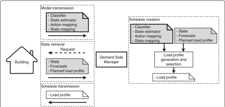
Fig. 1Provision and utilization of the flexibility model (cf. (Förderer et al.2018b)). Information generated by the EMS is depicted with a gray background and static information with an additional bold outline
for external influences are required. These variables are dynamic and sent periodically or requested when needed. In the state retrieval step depicted in Fig.1, the EMS transmits the load profile it has planned for the building to the DSMgr. This load profile is optional and may be used to determine the flexibility in the terms of deviations. With all this infor-mation the DSMgr is able to generate feasible load profiles, conduct a directed search for load profiles beneficial for their goals, or do a combination of both. The employed algo-rithm uses the process outlined in the “Process for generating load profiles” section. The best load profile according to the objective of the DSMgr is selected and then sent to and realized by the building’s EMS. A feedback mechanism for approving the schedule could easily be added.
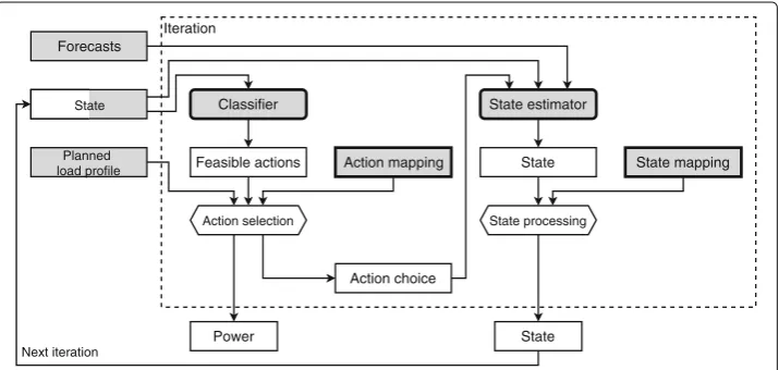
The central components of the presented approach are the classifier and the state estimator. There are several options for designing these components. For example, as discussed in “Related work”, equations and inequalities can be used to encode a Markov model or finite state machine. In this paper, theclassifierand thestate estimatorare both ANNs. With their help, the load profile is created element by element in a sequential pro-cess. The repeated estimation of the system’s state by thestate estimatormakes the ANN a recurrent neural network (RNN). Of course, a single RNN could have been used to com-bine theclassifierandstate estimatorwithin a single neural model, e.g., by embedding the feasible actions into the state space. However, we decided to stick to the generic structure depicted in Fig.2.
Process for generating load profiles
Forecasts
Classifier
Feasible actions
State estimator
Action choice
Power Iteration
State
Planned load profile
Action selection
Action mapping
State processing
State mapping
Next iteration
State
State
Fig. 2 The algorithm employed by the DSMgr iteratively determines a load profile using the model, parameters and variables provided by the EMS of the building. All data supplied by the EMS of the building is illustrated with a gray background and static information is additionally depicted with a bold outline
a feasible action is use case specific. Generally an action is considered feasible when the assigned rating exceeds a predefined threshold. When only taking the aggregated load of the building into consideration, action choices are based on the associated consumption or production of electricity. Actions could, for instance, be selected in a greedy fashion, trying to minimize the distance to a target load profile. Additional information like costs resulting from implementing certain actions could also be taken into account. The aver-age power consumed or produced by the building during periodtwhen implementing the selected, feasible actionatis given byl(at)and stored by the search algorithm. Given atthe estimate of the subsequent stateˆst+1=f(st,at,yˆt)is computed using thestate esti-mator f(·)and the forecastsˆytprovided by the building’s EMS. In some cases it may be beneficial to introduce a postprocessing step to correct some of the errors introduced by thestate estimator. This optional step uses thestate mapping p(·). In subsequent itera-tions the state resulting from the previous iteration ˆst+1is used as an input instead of the states0 sent by the EMS of the building. The resulting load profile is given by the sequence of power values(l(a0),. . .,l(aT−1))resulting from theaction selection. Devices that simply follow a fixed load profile once activated can be represented by encoding the load profile into a set of actions. Alternatively,l(·)could be adapted to include informa-tion about future periods that is added to subsequent values. After a feasible load profile has been identified, the process may either be restarted from scratch to compute a com-pletely new load profile or at any previously computed state in order to adapt the load profile starting from the respective iteration.
Dead ends and artificial constraints
this case, the load profile generation needs to be restarted from a period before reach-ing this dead end. Such situations may be avoided by introducreach-ing additional constraints or by converting hard constraints to soft constraints. In our example, there could be an additional (hard) constraint requiring a given minimum SOC of the HWT for the CHP plant to be able to shut down. By adapting the lower boundary according to the predicted heat demand, the described dead end can be avoided. In the following, we refer to such additionally introduced hard constraints as artificial constraints. Artificial constraints are introduced to shape the space of feasible load profiles and may require adding further elements to the state vector. How these constraints are derived and whether or not an adaptation of the state space is required is case specific.
Data acquisition
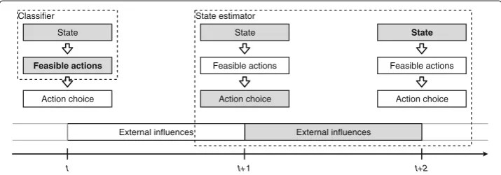
To train theclassifierand thestate estimator, data of feasible actions and state transitions are required. These data may be captured from real physical devices or generated by sim-ulation models. Figure3shows which data is required to train theclassifierand thestate estimatorrespectively, and when this data can be collected. The boldface elements are the respective models’ outputs. At the discrete point in timet, the real or simulated build-ing determines its current state and evaluates the available operational choices, i.e., the feasible actions, to choose an action. In order to train theclassifier, states and sets of fea-sible actions for many different points in time need to be collected. The subsequent state results from the building’s dynamics and is depending on the state, the chosen action and other external influences like the local consumption of energy or the solar irradiation. Hence, all of these are required to train thestate estimator.
When using data of a real building, the most important requirement is that the data needs to cover a sufficiently large range of system states. States that are never reached in the records, although technically attainable, will not be correctly represented in the result-ing flexibility model. A simulation model, on the other hand, can easily provide diverse states.
Implementing a simulation model specifically for training another model raises the question why this exact simulation model can not be given to the DSMgr in the first place. As we pointed out before, using equations and inequalities for theclassifierandstate esti-matorinstead of machine learning based models is indeed possible with our approach. The main motivation in seeking the utilization of machine learning models lies in the
External influences
t t+1
State
Action choice Feasible actions Classifier
State
Action choice Feasible actions
External influences
t+2 State
Action choice Feasible actions State estimator
potential of learning aggregated models. As we show in this paper, it is possible to learn a model of an aggregated system. In theory, larger aggregated models can be trained from individual models, by executing the process described inProcess for generating load pro-filesand collecting the required data depicted in Fig.3. When actions are defined on the basis of consumed and produced power, the aggregated model may simply reuse the exact same set of actions. Hence, in this case, only the dimension of the state space grows. Also, when defining actions in such a way, theaction mappingis only required if soft constraints need consideration. Furthermore, using ANNs may help to obscure some of the processes happening in the building. However, this is by no means guaranteed.
Simulation models and parameters
All data used to train the neural models is generated during the training process using simulation models. The simulation models emulate the represented systems starting from a randomly selected initial state. In each simulation step the set of feasible actions for the current system state is determined and an action is chosen randomly. Each sample for training theclassifieris generated from a single simulation period. Although we use single periods as samples for training thestate estimatorin this paper, a sample may also comprise a sequence of simulation steps to allow unfolding the recurrent neural model (see Goodfellow et al. (2016) for more information on unfolding RNNs).
Considered building configurations
In this paper three building configurations are considered. Each configuration is different in terms of the state space, the set of possible actions, as well as the associated restrictions and parameters the neural models need to learn from the data. A detailed description of the simulation models can be found in the subsequent sections. The following list provides an overview of the investigated configurations:
BESS: The state of the BESS is given by its SOC. Each action is uniquely associated with a power consumed or provided by the BESS. Hence, whether an action is feasible or not depends solely on the SOC of the BESS. The minimum and maxi-mum power are assumed to be constant. Charging and discharging efficiencies are considered.
CHP plant with HWT: The basic state is defined by the current mode of operation of the CHP plant, the dwell time and the temperature of the HWT encoded as SOC. Additional state variables have been introduced to configure constraints and prevent states without feasible actions. Only the two modes “off ” and “on” with fixed pow-ers are considered. After switching its mode of operation, the CHP plant needs to spend a certain time in the respective mode before the mode may be changed again. Whether an action is feasible or not is also dependent on the HWT’s SOC. Further-more, the ramping of the CHP plant and the heat loss of the HWT are considered in the state computation.
Aggregated system: The aggregated system, i.e., a BESS in combination with a CHP plant and a HWT, combines both of the above configurations.
Simulation models
BESS
One of the simplest options to define the state of the BESS is the amount of stored energy or equivalently the SOC. In the model, the SOC is computed in terms of the BESS’s usable capacity, i.e., the BESS may be discharged to an SOC of 0 and charged up to an SOC of 1. The amount of energy in the BESS at the beginning of periodtis given byet. When charging or discharging with powerpt over the length of a periodtthe change in the stored amount of energy (before loss) is
et=
ηcp
tt ,pt≥0 1
ηdptt ,pt<0
(1)
with charging and discharging efficienciesηcandηd. Each possible choice for the power
ptis equivalent to an action. For the loss, we distinguish a base loss that is equal to the loss at an SOC of 0 and a relative loss that is proportional to the SOC. As the SOC can not fall below 0 for a feasible load profile, this allows an intuitive state transition equation. The relative losslr is the percentage of stored energy that is lost every period. It is assumed that the stored energy changes linearly over the course of a period. The base losslbis a fixed amount of energy that vanishes every period. With these losses the amount of stored energy int+1 is given by
et+1=et+et−
et+et+1
2 ·l
r−lb
et+1=
et·
1− l r
2
+et−lb 1+ lr
2
.
(2)
Please note the occurrence ofet+1on both sides of the first line, as the loss is based on the average SOC. It islr = lb =0 for the BESS, but the same equations are used for the HWT. For identifying feasible actions the computation steps are simply reversed. From Eq.2it is
et=et+1·
1+l r
2
−et·
1− l r
2
+lb. (3)
By settinget+1to 0 and then to the amount of energy equivalent to an SOC of 100%, the minimum and the maximumetare derived. In combination with Eq.1the minimum and maximum power can be computed. By filtering out all actions exceeding one of these bounds, only feasible actions remain. The feasible actions are then stored in a list. In the simulation, theaction selectionfor the BESS is performed randomly with uniformly distributed probabilities to create equal amounts of samples for each action.
CHP plant with HWT
may only run if the SOC does not exceed 100% and it must run if the stored amount of thermal energy is not sufficient for satisfying the building’s thermal energy demand.
Similar to the BESS, the state of the HWT is computed with Eqs.1,2and3. As stated before, although included in the model, the parameters of the BESS have been chosen to neglect self-discharge. For the HWT, on the other hand, we neglect the efficiencies and consider self-discharge instead.
Since the CHP plant may only be turned off and on, there are only two actions available. Due to the combination of minimum dwell times for the CHP plant and the SOC limita-tions, there may arise situations without any feasible action as described in the “Dead ends and artificial constraints” section. To avoid this problem we introduce additional, artifi-cial minimum and maximum SOCs for the HWT. The CHP plant may only be started if the SOC is below its imposed maximum and only be stopped for an SOC above the minimum. Given suitable boundaries, dead end situations can be avoided. There are of course other possibilities to resolve this issue. In summary, including the additional vari-ables, the state is given by the current operation mode of the CHP plant, the dwell time in this mode, the minimum dwell times for each mode, the SOC of the HWT, and the min-imum and maxmin-imum HWT SOC. Whether an action is feasible or not is determined by the dwell time and the SOC in relation to the given boundaries. Again, for each iteration, feasible actions are stored in a list. Theaction selectionin the simulation is random.
Aggregated system
The aggregated system combines both simulation models described above. Hence, the state of the system is given by the SOC of the BESS, the current CHP plant operation mode, the dwell time in this mode, the minimum dwell times for each mode of the CHP plant, the SOC of the HWT, and the minimum and maximum HWT SOC. For our experiments, the set of possible actions for the aggregated system is simply the Cartesian product of both individual sets of possible actions. In consequence, there are multiple actions associated with the same aggregated building load. As the DSMgr aims to steer this aggregated load, identical actions in terms of resulting power consumed or produced could have been compared to remove the less desirable actions and reduce the amount of overall possible actions (see also “Data acquisition”).
Simulation model parameters
An overview of the model parameters is given by Table1. The parameters for the simu-lated BESS and CHP plant have been scaled in order to generate values from the intervals [−1, 1] and [ 0, 1] for the respective DER’s power. Thermal demand, as well as the param-eters for the HWT have been divided by 6 and thereby scaled accordingly. Originally, the HWT has a capacity of about 18 kWh which is roughly equivalent to a tank volume of∼780 l with temperatures ranging from 60° to 80 °C and 20 °C environmental tem-perature. The losses in W of a HWT with energy efficiency class B and volume V in liters are in [ 8.5+4.25·V0.4, 12+5.93·V0.4)(European Union2013). WithV =780 l and the normalization, the losses are in the interval [ 11.58, 16.18). Assuming a linear relationship between the SOC of the HWT and the heat losses, the total heat loss per simulated period is set to 11.58+SOC·(16.18−11.58)W. Thermal demand time series for a day in winter, summer, and the intermediate seasons, have been generated using the
Table 1Overview of the model parameters. The parameters for the BESS and the CHP plant have been normalized individually. Thermal consumption, the hot water tank capacity, and losses have been divided by 6 in order to scale them to a size appropriate for the normalized CHP plant
Parameter Normalized values
BESS Power el. [−1, 1] kW in steps of 0.01 kW
Capacity 1 kWh
Efficiency ηc=ηd=0.94
0.8836 round-trip efficiency
CHP plant Power el. 0 kW or 1 kW
Power thermal 0 kW or 1 kW
HWT Capacity 3 kWh
Heat loss 11.58+SOC·(16.18−11.58)W
Energy efficiency class B (European Union2013)
Thermal demand Winter 9.99 kWh/day
Intermediate 7.82 kWh/day
Summer 3.10 kWh/day
consumption patterns. Table 1 shows the normalized total demand. Each of the three series is the average of 60 simulations of identical four person households on a weekday and has a temporal resolution of one minute. Although the simulation models and the neural models use intervals of 15 min, the series are not aggregated. Instead, new ther-mal energy demand series are created by randomly selecting one value out of each 15 min period.
Neural models
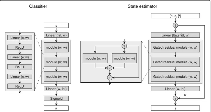
Since we use a rather arbitrary structure for the neural networks, it is very likely that there are more specialized ANNs that can achieve even better results. The structure of both neural models is depicted in Fig.4. Both models use a linear layer with biases for
Linear (w,w)
ReLU
Linear (w,w)
ReLU
Linear (w,w)
ReLU
module (w, w) module (w, w)
module (w, w) Linear (|s|, w)
Linear (w, |a|) s
Classifier State estimator
Gated residual module (w, w) module (w, w)
Gated residual module (w, w) Linear (|[a,s,y]|, w)
Linear (w, |s|) s [a, s, y]
s module (w, w)
×
+
1 Gated residual module (w, w)
+ 1
a Sigmoid
^
^
changing the number of elements in the input vector tow. This is followed by a sequence of modules consisting of other ANN layers. In theclassifiersuch a module consists only of linear layers with biases and rectified linear units, i.e.,ReLU(x) = x+ = max{x, 0}. The state estimator makes use of a more complexgated residual modulewhich in its structure is similar to a layer of the WaveNet (van den Oord et al.2016): The outputs of two modules are multiplied elementwise. Thereby one of the modules acts as a gate which can remove elements from the other module’s output by choosing a value of 0. Then, a residual connection adds the input of the modules to the result of the multiplication. The advantage of such a residual module is that its influence on the output can more easily be eliminated by the training algorithm (He et al.2016), which is especially relevant if the module is not needed. The number of modules determines the depth of the neural network and can be adapted using a hyperparemeter. Finally, a linear layer with biases is used to change the number of elements fromwto the desired output vector size. The sigmoid activation function isSigmoid(x)= 1+e1−x.
Aside from the structure of the ANNs, there are countless (hyper-)parameters to opti-mize and approaches to consider when training ANNs, including the selection of the optimization algorithm, loss function, i.e., the objective optimized by the training algo-rithm, batch size and learning rate. The models for theclassifierandstate estimatorare trained separately. In both cases the algorithm Adam (see Goodfellow et al. (2016)) is used for optimizing the neural models. The learning rate is adapted dynamically, based on the observed losses from previous batches and the number of training iterations. As is recommended in Goodfellow et al. (2016), a regularization term is introduced to the loss function to force smaller ANN weights. The term consists of the sum of the absolute model weights and is multiplied with a factor allowing to configure the impact of the reg-ularization. Additionally, norm clipping is used to prevent too large optimization steps (Goodfellow et al.2016). The source code and training logs that are published alongside the models provide a deeper insight into the employed regularization techniques and the parameter choices for the individual results.
Classifier
Given solely the state of the building and its DERs st as input, theclassifier computes a vector containing ratings for every action in the set A. These |A| ratings from the interval [ 0, 1] may be interpreted as the probability of feasibility for each individual action. For the three DER configurations BESS, CHP plant with HWT, and aggregated system, there are 1, 8, and 9 elements in st respectively (see Simulation models). For the creation of training samples, the simulation model and randomly selected initial states s0 are used to generate vectors for each state, indicating the feasibility of each action. Whether an action is feasible or not is encoded with 0 and 1, where a value of 1 denotes feasible actions. The target function for training the ANN is the binary cross entropy.
State estimator
weights provides a leverage for reducing the loss significantly by providing more precise forecasts for that respective element. Furthermore, although the inputs are all from the interval [ 0, 1], not every element in the state vector needs to be forecasted with exactly the same precision, especially since we apply a discretization as is described inDescribing and exploiting flexibility.
Evaluation setup
To evaluate the approach for generating feasible load profiles presented in this paper, neural models for theclassifierandstate estimatorare trained as described in the previous sections and tested in the process depicted in Fig.2. The goal of the evaluation is to show that the approach combined with ANNs can be used to reliably generate feasible and diverse load profiles, preferably from the entire space of feasible load profiles. We used
python withpytorch 1.0.1 for the implementation of all necessary models and scripts. During the training process, training batches are randomly generated with the help of the simulation models. In the evaluation, load profiles for one day with a temporal resolution of 15 min, i.e., consisting of 96 values, are generated using the presented approach in combination with the trained ANNs. With the simulation models used to generate the training samples, the generated load profiles are then evaluated for their actual feasibility. This section outlines the implementation of the remaining components in Fig.2needed in order to evaluate the approach.
Forecasts and initial states
For the load profile generation, thermal energy demand forecasts are generated from the data already used in the simulation models. All forecasts are assumed to be perfect. The load profiles planned by the EMS have not been used in the evaluation, since they are an optional element and the goal is to evaluate the feasibility of the presented approach. The initial states are selected randomly from the possible initial states used in the simula-tion model. In order to take varying thermal demand into account, the randomly selected artificial SOC bounds of the HWT are adapted according to the season. For winter, the intermediate seasons, and summer, the lower bound is at least 0.25, 0.2, as well as 0.15, and the upper bound is at most 0.85, 0.8, as well as 0.75. These exact bounds are an arbi-trary choice, considering only that there is a relationship between the season and thermal demand. In practice, the EMS of the building would adapt these bounds to reflect the forecasted demand.
Action selection
leads to the dead end statesthas to be considered infeasible and the process needs to be (partially) repeated from a statesτinτ <t.
In states close to boundaries imposed by constraints, small estimation errors may suf-fice to make a generated load profile infeasible, leading to an invalid load profile that is very similar to a feasible one. A possible solution to deal with this issue is the utilization of buffers. For the two configurations including a CHP plant and HWT, a buffer is added to the minimum and maximum HWT SOC values in the state vector. This is equivalent to further restricting the allowable HWT SOCs by tightening the artificial HWT con-straints. With this buffer, some of the actions near the feasibility boundary are ruled out to increase the likelihood of selecting feasible actions. The changes are applied to the state vector before passing it to theclassifier. The buffer is not applied in thestate estimation
or simulation models. Hence, the number of false negatives increases with an increasing buffer. Please note that for simplicity Fig.2does not include this additional preprocessing step.
After all actions likely to be feasible have been determined, an action needs to be selected. This is done randomly, drawing from a uniform distribution. A real DSMgr would rather conduct a targeted search and select the actions based on theaction mapping
and the target function to find a (nearly) optimal solution.
State processing
Even though thestate estimatormay generate good results during the training, estimating multiple steps may lead to growing errors. To counter this, in thestate processingstep, the state vector is discretized as described in “Describing and exploiting flexibility” section.
Results
The complete implementation of all simulation and neural models, the training and eval-uation algorithms, as well as the presented ANNs with the respective training logs and results have been published (see “Availability of data and materials”).
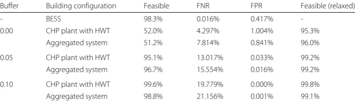
For each building configuration and different buffer sizes 1000 load profiles were gen-erated. A summary is shown in Table2. The false negative rate (FNR) and false positive rate (FPR) of the action classification strongly depend on the selected threshold for fea-sibility and the size of the buffer. As described earlier, the threshold has been set to 0.95 to ensure a low rate of false positives, since a false positive may invalidate a load profile, while a false negative only narrows the available flexibility. Buffers are only applied to the additional, artificial constraints for the HWT SOC. Since the buffers are applied to the
Table 2Feasibility and classification results for each configuration, based on 1000 individually generated load profiles
Buffer Building configuration Feasible FNR FPR Feasible (relaxed)
- BESS 98.3% 0.016% 0.417%
-0.00 CHP plant with HWT 52.0% 4.297% 1.004% 95.3%
Aggregated system 51.2% 7.814% 0.841% 96.0%
0.05 CHP plant with HWT 95.1% 13.017% 0.033% 99.2%
Aggregated system 96.7% 15.554% 0.016% 99.2%
0.10 CHP plant with HWT 99.6% 19.779% 0.000% 99.8%
classifierinput, the classification result contains an increased amount of false negatives compared to the actual target vector. For the BESS 98.3% of the generated load profiles are feasible, even without applying any buffers. In contrast, when no buffers are used, the models for the configurations including a CHP plant and HWT only generate about 50% feasible load profiles. As the buffer increases, the percentage grows. It may be surprising that there are infeasible load profiles when using a buffer of 0.1 even though there are no false positives. This is caused by situations where no action can be identified as valid option. Since we assume that there is always at least one feasible action, the action with the highest rating was chosen, even though there was no action rated above the threshold. For the configurations including a CHP plant and HWT, infeasibility is often caused by inaccurate HWT SOC estimations. Since the maximum and minimum SOC boundaries are artificially narrowed down to avoid dead ends, the resulting load profile may violate these artificial constraints while satisfying all real constraints. To determine the share of load profiles that satisfy the actual constraints, we remove the artificial SOC limitations after the load profile has been generated. The results for these relaxed constraints are given in Table2. Even without buffers, which in this case simply further narrow the artifi-cial boundaries, over 95% of the generated load profiles would actually be attainable. For increasing buffers, the percentage again increases. As mentioned before, a smart selec-tion process for the boundaries could help to further improve the results. Judging from the results, by applying similar artificial constraints to the BESS the rate of feasible load profiles could easily be increased to over 99%.
It is important to note that while the artificial constraints, buffers and high threshold for classifying actions as feasible help to increase the share of attainable load profiles, they also restrict the search space, i.e., the space of load profiles that can be generated. For larger buffers and more artificial constraints, a growing number of actually feasible load profiles is ruled out. The results for the BESS show that high shares of feasible load pro-files can indeed be achieved without artificial constraints and buffers. While the artificial HWT SOC constraints were introduced to avoid dead ends and the need for restarting the generation process, the introduction of buffers for the classifier was primarily motivated by the poor performance of the ANNs in states close to multiple boundaries at once. By improving the employed models or assuming a slightly different set of constraints, buffers may not be needed anymore for the CHP plant with a HWT.
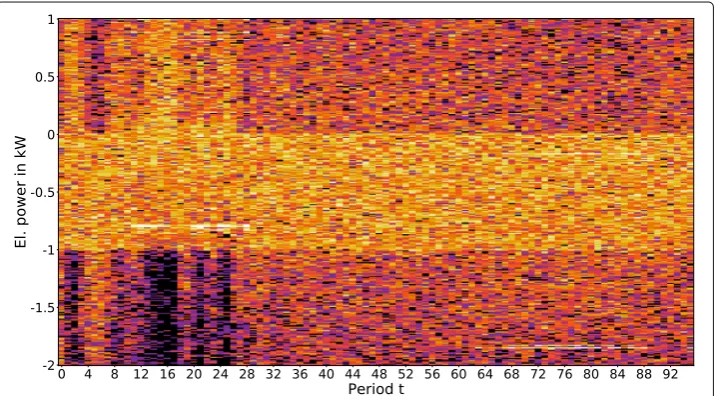
Fig. 5 Heat map indicating the coverage of all possible electric powers by the 997 generated load profiles. The more load profiles include a specific power value at a given period, the brighter the respective area. Black areas are reached by none of the 997 load profiles
diverse, as in every period t the majority of possible values is attainable with at least one load profile. In the early periods, there are some areas that are only covered by few load profiles. Similar areas show up when changing the initial state or the random seed for the random selection of the actions. These sparely covered regions are the result of high HWT SOCs. As more time passes, the underlying SOCs become more evenly distributed.
As depicted in Fig.4, thestate estimatorand theclassifierboth consist of a sequence of modules. While the implemented source code allows up to five modules, the presented results have been generated with ANNs using three modules at most. Even though those unused modules are included, each neural model that has been trained is less than 1 MiB in size. Removing the unused modules would lead to sizes of a few 100 KiB. To put this number into perspective, the dataset for the aggregated system has 2.564.776.224 possible states.
Conclusion
The approach presented in this paper enables the generation and directed search of load profiles for DERs. The employed models are used to perform an approximate simulation of the represented systems without the need of detailed knowledge of the systems them-selves. Since operational choices can easily be evaluated during the sequential process, a targeted load profile search is enabled. As the results show, we were able to generate diverse load profiles with a high likelihood of being feasible, not only for single DERs, but also for aggregates of multiple DERs. Hence, the presented approach could benefit demand side management measures by providing detailed information on the flexibility of diverse DERs.
Aside from the general applicability, we showed how additional constraints and buffers may be used to further increase the rate of feasible load profiles at the cost of narrowing the search space. Whether such restrictions of the search space pose an issue or not and how they should be designed needs to be assessed on a case-by-case basis. All code nec-essary to train own models and test the load profile generation has been published online, including the presented simulation and neural models, as well as the training logs and results (see “Availability of data and materials”).
In the future, we will continue to work on the approach by improving the ANNs, as well as the training process, by adding more DERs, and by evaluating and comparing the approach with others in a realistic scenario. Also, the field of reinforcement learning could provide beneficial ideas and concepts to further improve the approach, especially when using a state and action definition that does not require a separate classifier, e.g., when embedding feasible actions into the state. Moreover, the aggregation of multiple models to a combined model is a topic of interest, as it potentially enables large scale applications of the approach.
Acknowledgements
The authors would like to thank the anonymous referees for their valuable reviews and helpful suggestions.
About this supplement
This article has been published as part ofEnergy InformaticsVolume 2 Supplement 1, 2019: Proceedings of the 8th DACH+ Conference on Energy Informatics. The full contents of the supplement are available online athttps:// energyinformatics.springeropen.com/articles/supplements/volume-2-supplement-1.
Authors’ contributions
KF conceived and designed the research, implemented the models, and drafted and refined the manuscript. HS provided feedback, supervision, organization of funding and resources. Both authors have read and approved the final manuscript.
Funding
We gratefully acknowledge the financial support from the Federal Ministry for Economic Affairs and Energy (BMWi) for the project C/sells (funding no. 03SIN121). Publication of this supplement was funded by Austrian Federal Ministry for Transport, Innovation and Technology.
Availability of data and materials
Source code, data and trained models have been published, and are available on GitHub:https://github.com/kfoerderer/ State-Based-Load-Profile-Generation.
Competing interests
The authors declare that they have no competing interests.
Author details
1FZI Research Center for Information Technology, Haid-und-Neu-Str. 10–14, 76131 Karlsruhe, Germany.2Karlsruhe Institute of Technology, Kaiserstraße 12, 76131 Karlsruhe, Germany.
References
Abuella M, Chowdhury B (2015) Solar power forecasting using artificial neural networks. In: 2015 North American Power Symposium (NAPS). IEEE. pp 1–5
Akkaya I, Fremont DJ, Valle R, Donzé A, Lee EA, Seshia SA (2016) Control improvisation with probabilistic temporal specifications. In: 2016 IEEE First International Conference on Internet-of-Things Design and Implementation (IoTDI). IEEE. pp 187–198
Batra N, Kelly J, Parson O, Dutta H, Knottenbelt W, Rogers A, Singh A, Srivastava M (2014) Nilmtk: An open source toolkit for non-intrusive load monitoring. In: Proceedings of the 5th International Conference on Future Energy Systems. e-Energy ’14. ACM, New York. pp 265–276
Bremer J, Rapp B, Sonnenschein M (2010) Support vector based encoding of distributed energy resources’ feasible load spaces. In: 2010 IEEE PES Innovative Smart Grid Technologies Conference Europe (ISGT Europe). IEEE. pp 1–8 Bremer J, Rapp B, Sonnenschein M (2011) Encoding distributed search spaces for virtual power plants. In: 2011 IEEE
Symposium on Computational Intelligence Applications In Smart Grid (CIASG). IEEE. pp 1–8
Bremer J, Lehnhoff S (2017) Hybrid multi-ensemble scheduling. In: Squillero G, Sim K (eds). Applications of Evolutionary Computation. Springer, Cham. pp 342–358
Bremer J, Lehnhoff S (2018) Phase-space sampling of energy ensembles with cma-es. In: Sim K, Kaufmann P (eds). Applications of Evolutionary Computation. Springer, Cham. pp 222–230
Bremer J, Sonnenschein M (2013a) Constraint-handling for optimization with support vector surrogate models - A novel decoder approach. In: Filipe J, Fred ALN (eds). ICAART 2013 - Proceedings of the 5th International Conference on Agents and Artificial Intelligence, Volume 2, Barcelona, Spain, 15-18 February, 2013. SciTePress, Setúbal. pp 91–100 Bremer, J, Sonnenschein M (2013b) Model-based integration of constrained search spaces into distributed planning of
active power provision Vol. 10. pp 1823–1854
Costanzo GT, Zhu G, Anjos MF, Savard G (2012) A system architecture for autonomous demand side load management in smart buildings. IEEE Trans Smart Grid 3(4):2157–2165
Nieße A, Sonnenschein M, Hinrichs C, Bremer J (2016) Local soft constraints in distributed energy scheduling. In: 2016 Federated Conference on Computer Science and Information Systems (FedCSIS). IEEE. pp 1517–1525
European Union (2013) Commission Delegated Regulation (EU) No 812/2013 of 18 February 2013 supplementing Directive 2010/30/EU of the European Parliament and of the Council with regard to the energy labelling of water heaters, hot water storage tanks and packages of water heater and solar device Text with EEA relevance. Off J Eur Union L 239:83–135
Förderer K, Ahrens M, Bao K, Mauser I, Schmeck H (2018) Modeling flexibility using artificial neural networks. Energy Inform 1(1):21
Förderer, K, Ahrens M, Bao K, Mauser I, Schmeck H (2018) Towards the modeling of flexibility using artificial neural networks in energy management and smart grids: Note. In: Proceedings of the Ninth International Conference on Future Energy Systems. e-Energy ’18. ACM, New York. pp 85–90
Goodfellow I, Bengio Y, Courville A (2016) Deep Learning. MIT Press, Cambridge.http://www.deeplearningbook.org
Graßl M, Vikdahl E, Reinhart G (2014) A petri-net based approach for evaluating energy flexibility of production machines. In: Zaeh MF (ed). Enabling Manufacturing Competitiveness and Economic Sustainability. Springer, Cham. pp 303–308 He K, Zhang X, Ren S, Sun J (2016) Deep residual learning for image recognition. In: 2016 IEEE Conference on Computer
Vision and Pattern Recognition (CVPR). IEEE. pp 770–778
Hoogsteen G, Molderink A, Hurink JL, Smit GJM (2016) Generation of flexible domestic load profiles to evaluate demand side management approaches. In: 2016 IEEE International Energy Conference (ENERGYCON). IEEE. pp 1–6
MacDougall P, Kosek AM, Bindner H, Deconinck G (2016) Applying machine learning techniques for forecasting flexibility of virtual power plants. In: 2016 IEEE Electrical Power and Energy Conference (EPEC). IEEE. pp 1–6
Malbasa V, Zheng C, Chen PC, Popovic T, Kezunovic M (2017) Voltage stability prediction using active machine learning. IEEE Trans Smart Grid 8(6):3117–3124
Mauser I, Müller J, Förderer K, Schmeck H (2017) Definition, modeling, and communication of flexibility in smart buildings and smart grids. In: ETG-Fb. 155: International ETG Congress 2017. VDE, Berlin. pp 605–610
McKenna E, Thomson M (2016) High-resolution stochastic integrated thermal-electrical domestic demand model. Appl Energy 165(Supplement C):445–461
McLoughlin F, Duffy A, Conlon M (2010) The generation of domestic electricity load profiles through markov chain modelling. Euro-Asian J Sustain Energy Dev Policy 3
Neugebauer J, Bremer J, Hinrichs C, Kramer O, Sonnenschein M (2016) Generalized cascade classification model with customized transformation based ensembles. In: 2016 International Joint Conference on Neural Networks (IJCNN). IEEE. pp 4056–4063
Neugebauer J, Kramer O, Sonnenschein M (2015) Classification cascades of overlapping feature ensembles for energy time series data. In: Woon WL, Aung Z, Madnick S (eds). Data Analytics for Renewable Energy Integration. Springer, Cham. pp 76–93
Neugebauer, J, Kramer O, Sonnenschein M (2017) Instance Selection and Outlier Generation to Improve the Cascade Classifier Precision. In: van den Herik J, Filipe J (eds). Springer, Cham. pp 151–170
Rashid T, Huang B, Kechadi T, Gleeson B (2006) Auto-regressive recurrent neural network approach for electricity load forecasting. Int J Comput Intell 3(1):36–44
Rodrigues F, Cardeira C, Calado JMF (2014) The daily and hourly energy consumption and load forecasting using artificial neural network method: A case study using a set of 93 households in portugal. Energy Procedia 62:220–229. 6th International Conference on Sustainability in Energy and Buildings, SEB-14
Santo KGD, Santo SGD, Monaro RM, Saidel MA (2018) Active demand side management for households in smart grids using optimization and artificial intelligence. Measurement 115(Supplement C):152–161
Sawall H, Scheuriker A, Stetter D (2018) Flexibility Definition for Smart Grid Cells in a Decentralized Energy System. In: Proceedings of the 7th International Conference on Smart Cities and Green ICT Systems - Volume 1: SMARTGREENS. SciTePress, Setúbal. pp 130–139. INSTICC
Severini M, Squartini S, Fagiani M, Piazza F (2015) Energy management with the support of dynamic pricing strategies in real micro-grid scenarios. In: 2015 International Joint Conference on Neural Networks (IJCNN). IEEE. pp 1–8 Song J, Krishnamurthy V, Kwasinski A, Sharma R (2013) Development of a markov-chain-based energy storage model for
Sutton RS, Barto AG (2018) Reinforcement Learning: An Introduction. MIT Press, Cambridge.http://incompleteideas.net/ book/the-book-2nd.html
Tao L, Ma J, Cheng Y, Noktehdan A, Chong J, Lu C (2017) A review of stochastic battery models and health management. Renew Sust Energ Rev 80:716–732
van den Oord A, Dieleman S, Zen H, Simonyan K, Vinyals O, Graves A, Kalchbrenner N, Senior A, Kavukcuoglu K (2016) WaveNet: A Generative Model for Raw Audio. CoRR abs/1609.03499.http://arxiv.org/abs/1609.03499
Vázquez-Canteli JR, Nagy Z (2019) Reinforcement learning for demand response: A review of algorithms and modeling techniques. Appl Energy 235:1072–1089
Publisher’s Note
Springer Nature remains neutral with regard to jurisdictional claims in published maps and institutional affiliations.
Submit your manuscript to a
journal and benefi t from:
7Convenient online submission 7Rigorous peer review
7Immediate publication on acceptance 7Open access: articles freely available online 7High visibility within the fi eld
7Retaining the copyright to your article