Overlapping community detection for count-value networks

Overlapping community detection

for count‑value networks

QianCheng Yu

_{, ZhiWen Yu}

_{, Zhu Wang}

_{, XiaoFeng Wang}

_{and YongZhi Wang}

Introduction

Community detection is a fundamental problem in network analysis, as community structure which almost exists in all networks, is the most widely studied structural prop-erties of networks.

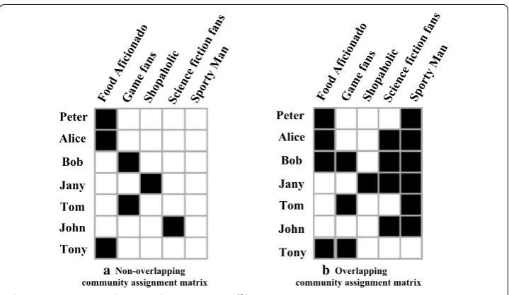
Statistical network generative model, due to its solid theoretical base, remarkable interpretability and relative tractability, has been wildly used for community detect-ing tasks [1]. Existing network generative models can be grouped into two classes: the latent class model, and the latent feature model. The latent class model assume that each individual only affiliate with a single class (as show in Fig. 1a). The latent feature model, increases the flexibility of the generative process by permitting each object possesses a vector of features and determine the link probabilities based on interactions among the features. In many real-world networks, communities are ordinarily overlapping rather than disjoint, so assuming that each object having hard membership in only one cluster became too restrict to consistent with the facts.

An important challenge in community detection is to specify the number of com-munities in advance, as we do not have good prior knowledge of how many parameters the model requires to explain the data well. The relational infinite latent feature model

Abstract

Detecting network overlapping community has become a very hot research topic in the literature. However, overlapping community detection for count-value networks that naturally arise and are pervasive in our modern life, has not yet been thoroughly studied. We propose a generative model for count-value networks with overlapping community structure and use the Indian buffet process to model the community assignment matrix Z; thus, provide a flexible nonparametric Bayesian scheme that can allow the number of communities K to increase as more and more data are encoun-tered instead of to be fixed in advance. Both collapsed and uncollapsed Gibbs sampler for the generative model have been derived. We conduct extensive experiments on simulated network data and real network data, and estimate the inference quality on single variable parameters. We find that the proposed model and inference procedure can bring us the desired experimental results.

Keywords: Overlapping community detection, Count-value networks, Generative network model, Nonparametric Bayesian model, Indian buffet process, Inference quality estimation

Open Access

© The Author(s) 2019. This article is distributed under the terms of the Creative Commons Attribution 4.0 International License (http://creat iveco mmons .org/licen ses/by/4.0/), which permits unrestricted use, distribution, and reproduction in any medium, provided you give appropriate credit to the original author(s) and the source, provide a link to the Creative Commons license, and indicate if changes were made.

RESEARCH

*Correspondence: [email protected]. edu.cn

†_{QianCheng Yu and ZhiWen} Yu contributed equally to this work

(rILFM), in which the number of latent variables is unbounded, is a flexible Bayesian nonparametric approach that is a proper choice for such situation, as its number of parameters can be vary along with the data increasing.

The Indian buffet process (IBP) [2] is often used to develop construction for the over-lapping community assignment matrix, in which each object is represented by a sparse subset of an unbounded number of features, thus can lead to a Bayesian nonparametric version of the latent feature model.

As show in Fig. 1b, the set of features possessed by a set of objects can be expressed in the form of a binary matrix Z with infinite columns and exchangeable rows, where the ith row is an object, and the kth column corresponds to a feature, zik indicates that object i possesses

feature k. The infinite binary matrix Z can describe that each individual is characterized by a set of features, or equivalently to say that each individual belongs to multiple communities simultaneously, which is intuitively named as overlapping community structure.

Most of the existing works represent a network as a symmetric binary adjacent matrix and a Bernoulli distribution (or a logistic Gaussian distribution) is chosen to formu-late the generative mechanism, for its simplicity. The symmetric binary adjacent matrix representation has two limitations: (1) when we transform these count-value networks into a symmetric binary adjacent matrix representation, we lose many valuable network information which can help to find overlapping community, e.g., if we use binary net-work, all nodes play equal roles in one community, as there only have two situations: linked or not linked; but, if we consider the interaction times between nodes, they are no longer play equal roles, the count vale may imply which nodes are at the core of one community, which are at the periphery. (2) The MCMC (Markov chain monte carlo) inference of the generative model with Bernoulli likelihood is difficult to derive.

It is well known to us that count-value networks naturally arise and are pervasive in our modern life. For example, in communicate networks, such as email networks, phone call networks, instant messaging networks, worker recruitment influence networks in mobile crowd sensing (MCS) platforms [3] etc., interactions are often directed and have an

Peter Alice Bob Jany Tom

Tony John Peter

Alice Bob Jany Tom

Tony John

Non-overlapping

community assignment matrixa community assignment matrixb Overlapping

associated count value, i.e., person i can send mails (make phone calls or send messages) to person j many times. On online social media service platforms such as Twitter, Facebook, BBS, and MCS [4], people follow (comment, like or reply to) those whom they are inter-ested in, such interactions also have direction and are associated with interaction times.

In this article,we concerned on overlapping community detection for count-value social networks. We propose a generative model for count-value networks with overlapping community structure: the network is modeled as a Poisson point process, after applying Poisson factor analysis on the corresponding count matrix, we obtain M=ZZT , which is akin to the mixed membership stochastic block model (MMSB) [5] that can express the overlapping community structure. The IBP is used as the prior to model the community assignment matrix Z; thus, allows the number of communities K to be determined at infer-ence time instead of to be predefined. Both a collapsed and an uncollapsed Gibbs sampler for the generative model have been derived. We reinforce the validity of the theoretical results via extensive experiments on simulated network data and real network data.

Related works

Following the seminal work of Erdos and Renyi [6], various random graph models have been proposed. The celebrated SBM (stochastic block model) [7] and its extensions such as the IRM (infinite relational model, Kemp et al. [8]), MMSB (Airoldi et al. [5]), DCSBM (degree-corrected SBM, Karrer et al. [9]), DSBM (dynamic SBM, Pensky [10]), have a wide variety of applications in network community detection, and form a huge corpus especially in social sciences and machine learning. We do not present an exhaustive review here; for an up-to-date account of various aspects, we direct the reader to Fortu-nato [11], Xie et al. [12] and Matias et al. [13] for reference.

There already have some pioneering works which composing the ideas of the classical MMSB model and the nonparametric Bayesian approach to increase the flexibility of net-work generative process by letting each node possess potentially infinite number of features, for example, the celebrated LFRM (latent feature relational model) proposed by Miller et al. [14], which was previously described in Meeds et al. [15]. The IMRM (infinite multiple rela-tional) model proposed by Morup et al. [16] is a variant of the LFRM model, in which a noisy-or likelihood was used instead of the logistic Gaussian likelihood. The ILA [17] (infinite latent attribute) model presented in Palla et al. (2015) generalized the LFRM mode by allow-ing an explicit representation of the partitionallow-ing of each general community into subclasses, thus providing a more structured representation of the data. All these models assume that K is not known a priori and use the IBP to account for the number of latent communities.

Although most of the existing work does not consider count-value networks, some research work provides an exception. For example, Karrer and Newman introduced the DCSBM model [9], they assumed that the links between nodes i and j follow a Poisson distribution and, thus, represented network as a count adjacent matrix. This method is reasonable, as the Poisson distribution is the natural probability distribution for modeling counts. Tue Her-lau et al. [18] formulated a nonparametric Bayesian generative model for the DCSBM (they named it IDCSBM), where the number of communities is inferred via the Chinese restaurant process [19]. These two models can be used to detect only nonoverlapping communities.

showing that it could be constructed from an exchangeable sequence of beta-Bernoulli processes. They further showed that the beta-Bernoulli process is the underlying de Finetti mixing measure for the IBP.

The Poisson factor model, which is also named the Gamma-Poisson model, is a proba-bilistic matrix factorization model that has been widely used in many areas such as image reconstruction, text information retrieval, and collaborative filtering etc.. The first applica-tion of Poisson factor analysis to network analysis was presented in Zhou et al. [21].

The proposed model

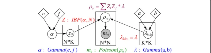
Let G=(V,E) denote a count-value graph, Gt=(Vt,Et) denote a network snapshot which was observed at time t. Vt= {v1,v2,. . .,vN} is node set of Gt , nodes often correspond to

persons or objects in network. N = |Vt| is the number of nodes. Et is the edge set, edges

often correspond to relationships between objects. Each observed edge inherently associ-ate with a count value mij . The dynamically evolving network G can be modeled using a random process, and this infinite random process can be decomposed into many observed network snapshots. Each network snapshot Gt is finite, so it correspond to an adjacent

matrix M which is a count-value matrix. The application of Poisson factor analysis to the random count matrix M, results in M=ZZT , where the N×K matrix Z is called the

community assignment matrix of the network, and the K×K square matrix is called the community compatibility matrix. In this case, we have

where zik1 expresses how strongly node i is affiliated with community k1 , and k1k2

measures how strongly communities k1 and k2 interact with each other. The product

z_ik1k1k2zjk2 measures how strongly nodes i and j are connected due to their affiliations with communities k1 and k2 respectively. One caveat here is that the infinite Gamma-Poisson model often use the multi-scoop IBP, which is a distribution over a random count matrix, as the prior of Z; but here we use the basic IBP which is a distribution over a random binary matrix.

The generative process of our model is as follow:

mij∼Poisson

K

k1=1 K

k2=1

z_ik1k1k2zjk2 , (1) P(M)= N

j=1 N

i=1

P(mij), mij∼Poisson(ρij)

mij= K

k1=1 K

k2=1

mik1k2j mik1k2j∼Poisson(k1k2)

ρij= K

k1=1 K

k2=1 _k

1k2 =ZiZj∗

Z=(Z1,. . .,ZN)T Z∼IBP(α,N) α∼Gamma(e,f)

P(�)= K

k1=1 K

k2=1

P(_k

Here, we let all _k

1k2 = , we will explain the reason in "Inference tricks" subsection . The

probability graph model representation for the generative process is depicted in Fig. 2. Apparently, the Poisson factor analysis, is guaranteed by the superposition principle of the Poisson point processes.

Superposition is an additive set operation such the superposition of a k-point configu-ration in Xn is a kn−point configuration in X. Examples of Poisson superposition pro-cesses include the compound Poisson, and the negative binomial propro-cesses.

Theorem 1 (Poisson Superposition Principle) Give k independent Poisson point pro-cesses�1,�2,. . .,�k, and the corresponding counting processes areN1,N2,. . .,Nk , which

with intensity measureµ1,µ2,. . .,µk, then= ∪k_i=1ialso is a Poisson point process, the corresponding counting process isN =k_i=1Ni , its intensity isµ=ki=1µi [22].

We apply the restriction that links are directly generated by individual features instead of through complex interactions between features, so that feature and community are the same concepts, i.e., stating that node i possesses feature j is equivalent to stating that node i is affiliated with community j.

As show in Fig. 1b, nodes are assigned to a set of communities can be expressed in the form of a binary matrix with infinite columns and exchangeable rows, where the ith row is the community assignment vector Zi of the node i, and the jth column corresponds to a community, zij=1 indicates that node i affiliated to community j. As Zi may has many

nonzero element, i.e. there is no assumption of mutual exclusivity and exhaust, thus the community affiliation matrix Z can characterize overlapping community structure in a network.

Parameter inference

The IBP is a distribution over an exchangeable binary matrix, it can be constructed in two ways, restaurant construction and stick-breaking construction. The former eas-ily lends itself to MCMC inference, and the latter easeas-ily lends itself to variational infer-ence [23]. Although the execution time required for MCMC inference is cubic due to the number of observations and thus often scales poorly [24], we can only use MCMC to infer the rILFM models if we do not want to predefine K because the stick-breaking construction of the IBP leads to a variational method for inference based on truncating to a finite model. Thus we must predefine the truncating level, which is as difficult as predefining K.

In this paper, we derived both a collapsed and an uncollapsed Gibbs sampler for Z. In "Uncollapsed Gibbs sampler" subsection, we illustrate the uncollapsed Gibbs sampler based

MCMC inference algorithm, and in "Collapsed Gibbs sampler" subsection, we depict details about derivation of the collapsed sampler.

Uncollapsed Gibbs sampler

Let M1 denote the set of observed links, (i,j)∈M1 means that there is a link between node i and j (in other word, mij>0 ), EV =(i,j)∈M1mij denote the total number of links,

C=n

i=1 n

j=1(ZiZj)=Z

ZT denote the total number of communities shared by

node pairs (i,j)∈M (

denote the Hadamard product operation on matrix), HN denote the harmonic number, Z−ik denote all community assignments except zik , knew denote new

sampled features for each object. The inference procedure of our model is as follow:

Algorithm 1:Uncollapsed Gibbs sampling procedure

Input: adjacent matrixM, total number of sampling iterationsmaxIter, number

- of burning samplesburnin

Output: samples draw from the posterior distribution overZ Algorithm step:

1. Initialize model parametersα, λ, Z

2. For each iteration iter= 0,1, ..., maxIter−1 :

- 2.1Uncollapsed Gibbs sampling updateZ

- (1.)ReshapeZ

- If there any column inZwhich is an all-zero column vector, delete it.

- (2.) For each object i= 1, ..., N :

- 1.) Update existing features: - For each featurek= 1, ..., K:

- Samplingzikfor existing features from distributionP(zik|.)∝P(M|Z, λ) - P(zik|Z−ik), whereP(zik= 1|Z−ik, M, λ)∝m_i−ik₁P(M|Z, λ)

- 2.) Determine number of new featuresknew

- Samplingknewaccording toP(knew)∝P oisson(knew;_Nα)P(M|Znew, λ), - whereZnew denote assignments of new features.

- 2.2Updateλ

- Sampling a newλaccording toλ∼Gamma(a+EV,1.0/(b+C))

- 2.3Updateα

- Sampling a newαaccording toα∼Gamma(e+K,1.0/(f+HN)

3. Throw those burning samples and outputmaxIter−burninsamples draw from - the posterior distribution ofZ.

In each sampling iteration, for each object, when we determine number of new features, the likelihood P(M|Znew,) is obtained by the integral

We need to perform a Monte Carlo integration to draw knew according to P(knew)∝Poisson(knew;_Nα)P(M|Znew,) . This procedure is equivalent to an importance

sampling procedure: first, we draw many pairs (knew,�new) , where new denote new part

�new

of which correspond to those new features. Then, assign a weight to each pair based on the data likelihood P(M|Znew,,�new) . Last, based on the weights,we sample a pair (knew,�new) and take its knew item as our knew.

Collapsed Gibbs sampler

Different from the uncollapsed Gibbs sampler, the collapsed Gibbs sampler use P(M|Z, a, b) as likelihood distribution instead of P(M|Z,) , and thus we need not to

update , i.e., step 2.2 in the Algorithm 1 can be omitted. As differences between the two

samplers are very clear, we have no need to illustrate the collapsed Gibbs sampler based MCMC inference algorithm, we just depict details about derivation of the collapsed sampler here.

First, we derive the likelihood distribution which was used in the uncollapsed Gibbs sampler. Let M0 denote the set of observed unlinks, (i,j)∈M0 means that there is no

link between node i and j (in other word, mij=0).

1. Derive the likelihood in the uncollapsed Gibbs sampler

As the likelihood distribution in the uncollapsed sampler is conjugate to the prior of

, we can integrate out to obtain the likelihood in the collapsed sampler.

2. Integrate out to obtain the likelihood in the collapsed sampler P(M|Z,)= �

(i,j)∈M1 ρ_ijmij

mij!

exp(−ρ_ij) �

(i,j)∈M0

exp(−ρ_ij)

= �

(i,j)∈M1 ρ_ijmij

mij! �

(i,j)∈M1

exp(−ρ_ij) �

(i,j)∈M0

exp(−ρ_ij)

= �

(i,j)∈M1 π_ijmij

mij! �

(i,j)∈M

exp(−ρij)

= �

(i,j)∈M1 (∗�

ZiZj)mij mij!

�

(i,j)∈M

exp�−�(ZiZj)∗ �

= �

(i,j)∈M1 (�

ZiZj)mij∗mij mij!

�

(i,j)∈M

exp�−�(ZiZj)∗ �

=� ��

ZiZj�mij mij!

∗�mij � (i,j)∈M

exp�−�(ZiZj)∗ �

= �

(� ZiZj)xij �

xij!

∗�mij_exp 

− �

(i,j)∈M �

(ZiZj)∗ 



= �

(� ZiZj)mij �

mij!

Inference tricks

In order to derive a feasible MCMC inference procedure, we make the following assumptions for our model:

1. We assume that is a diagonal matrix, links only exist between nodes in the same

community, i.e., there’s no link from a node in community k1 to a node in community k2 when k1! =k2;

2. We restrict all link probability _k

1k2 to take the same value , this means nodes within each community have same opportunity to form a link.

These two assumptions can bring us two benefits, one is that we don’t need to change the shape of along with the changes of K, the other is that we can obtain

the conjugacy between the likelihood and the Gamma prior for . Under this

circum-stance, can be integrated away and a collapsed Gibbs sampler for Z can be derived.

The IBP has a major weakness: the generated Z is determined only by N and α ,

regardless of the characteristics of the observations. For example, if node i is an iso-lated node, its community assignment vector should be an all-zero vector, but the IBP ignores this fact and assigns node i to some communities. Some steps are taken to correct this clear mistake and to avoid unnecessarily updating of the all-zero rows in Z. And accordingly make the MCMC inference accelerated.

1. Assign a flag to isolated node

We maintain a flag vector with all-zero initial values. First, we check each node in the graph. If its in-degree and out-degree both are zero, we set its flag to one to indicate that the node is not affiliated with any community;

2. Skip unnecessary update steps

After the initial Z has been generated, according to the flag, we change the

corre-sponding row in Z to an all-zero vector. In the process of each MCMC iteration,

when we update Z, if a node’s flag is one, we don’t update the corresponding row. P(M|Z,a,b)=

P(M|Z,)P(|a,b)d

=

(

ZiZj)mij

mij!

∗EV_exp(−C∗) b

a

Ŵ(a)

a−1

exp(−b)d

=

(

ZiZj)mij

mij!

ba

Ŵ(a)

a+EV−1_exp(−(b+C)_)d

=

₍

ZiZj)mij

mij!

ba

Ŵ(a)

Ŵ(a+EV) (b+C)a+EV

(b+C)a+EV

Ŵ(a+EV)

a+EV−1

exp(−(b+C))d

=

₍

ZiZj)mij

mij!

ba

Ŵ(a)

Ŵ(a+EV) (b+C)a+EV

=

₍

ZiZj)mij

mij!

baEV

After we perform posterior inference on Z, based on the assumption that a commu-nity should contain at least three nodes, we will cancel those columns in the inferred

Z which have less than three non-zero values.

Per‑iteration running times

For both the uncollapsed Gibbs sampler and the collapsed Gibbs sampler, when analysis algorithm complexity, we only consider the number of the Hadamard product operates on Z (i.e., element-wise matrix multiplication Z

ZT ) for one sweep through a N∗K community assignment matrix Z under a compound Poisson likelihood model.

The running time of both two Gibbs samplers are dominated by the computation of the likelihood. When we change one element of Z, the likelihood need to be calculated twice, thus Z may be updated in O(N3_{K) time.}

Experiments

We implemented our model and the inference algorithm using python. After we finished Bayesian analysis, the posterior which contains all the information about model param-eters according to the observed data and the model, was need to be summarized [25].

For single variable parameters such as α and , it is easy to communicate the result, as

the most probable posterior value is given by the mode of the posterior distribution (i.e., the peak of the distribution). It is also a good choice to report the mean (or median) of the distribution and some other measure, such as standard deviation or HPD (highest posterior density) interval, to have an idea of the dispersion and hence the uncertainty in our estimate [25].

Experiment on synthetic data

We analyzed one synthetic network generated according to our network gen-erative model. Because the ground truth is known, it is easy to empirically vali-date our theoretical findings. We generate synthetic data from the IBP prior (with

N=30,a=b=1,e=14,f =1/HN , α∼Gamma(e,f) , α=1.7658 ) and the

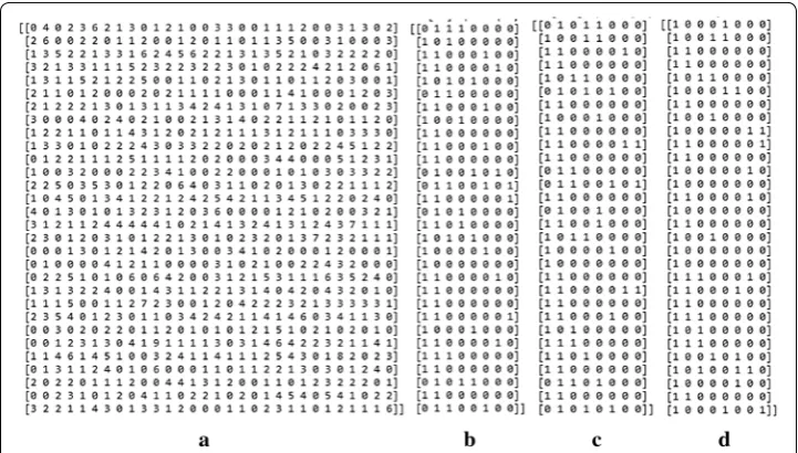
com-pound Poisson model (with ∼Gamma(a,b) , =0.3872 ). The simulated graph is a directed graph, with 30 nodes and 666 edges, its adjacent matrix M and community assignment matrix Z were depicted in Fig. 3a, b.

We ran six chains, among them: chain1, chain2 and chain3 correspond to the uncollapsed sampler (we use U stand for it), chain4, chain5 and chain6 correspond to the collapsed sampler (we use C stand for it). Among them, chain1 and chain4

start with a=b=1,e=4,f =1/HN , α=0.1543 ; chain2 and chain5 start with

a=b=1,e=14,f =1/HN , α=1.7658 , i.e., the ground truth of all parameters;

chain3 and chain6 start with a=b=1,e=24,f =1/HN , α=3.7991 . We ran each chain maxIter=10, 000 MCMC iterations, throw burnin=3000 samples and

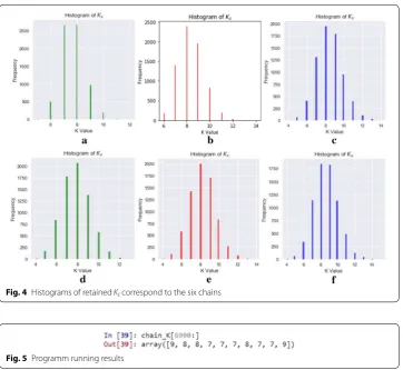
col-lected the last 7000 samples. We illustrate occurring times of all the Ks values sam-pled from the six chains in Table 1.

As depicted in Table 1 and Fig. 4, in all six chains, mode of Ks is 8, which is as same

dispersion on Ks value than chain4, chain5 and chain6. From this perspective, we

can draw a conclusion that uncollapsed samplers get better inference results than col-lapsed samplers. We also can see that when alpha takes a small value, samples with Ks=7 are more than samples with Ks=9 , when alpha takes a bigger value, the

num-ber of samples with Ks=9 become larger, i.e., the setting has big affect to the statisti-cal dispersion on K.

For structured parameters such as Zik s, the common practice to summarize it is to take the modulus of Ks as the K value and take the last sample as Z. Apparently, the chain1 did not has a good discrimination degree, because the number of samples with Ks=7 and Ks=8 are almost equal. So, we use the 6997th sample which was

drawn from the chain2 as our posterior inference result. See Fig. 5 for the programm running results.

The inferred Z was depicted in Fig. 3c. We compare the posterior inference results with the ground truth and the 1000th sample (which was depicted in Fig. 3d) via illustrate their communities in Table 2. The second row of Table 2 records the true communities, we can see that C1, C2,…, C8 are subset of Vt , and Ci Cj = ∅,∀i,j=1, 2,. . ., 8 , i.e., C1, C2,…, C8 are overlapping communities.

Fig. 3 a Depict the adjacent matrix M of the simulated graph, b depict its community assignment matrix Z, these are the ground truth. c depict the inferred Z via the uncollapsed sampler, which were obtained from chain2 in the 6997th MCMC iteration. d depict Z sampled from chain2 in the 1000th MCMC iteration

Table 1 Occurring times of all the Ks values sampled from six chains

Italic value indicates significance of Ks value

4 5 6 7 8 9 10 11 12 13 14 15

From Table 2, we can see that the biggest two communities C1 and C2 have the same objects in both the ground truth and the inferred results, but those small com-munities are different from each other. Only 6 objects v11,v18,v19,v22,v27,v29 have

the same community affiliation, imply that for an unsupervised learning task, such as overlapping community detection, even if we known the ground truth, it is hard to obtain accuracy results via statistical machine learning method. Let us see Z sampled from chain2 in the 1000th MCMC iteration, it is very far from the ground truth, so it’s necessary to throw the burning samples away.

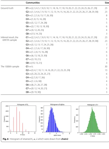
Compare the histogram of α (middle in Fig. 6) and the histogram of (right in

Fig. 6) correspond to the chain2, we found that the change range of α is larger, while that of is smaller.

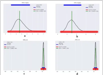
This conclusion can also be verified according to metrics depicted in Fig. 7, we can see that the HPD of (Fig. 7a) is more short of the HPD of α (Fig. 7b). The HPD is

the minimum width Bayesian credible interval, it is the shortest interval containing a given portion of the probability density. One of the most commonly used is the 95% HPD or 98% HPD, often accompanied by the 50% HPD.

In Fig. 7, the black curve describes the posterior using a kernel density estimation, mode, ROPE means lower and upper values of the region of practical equivalence. When we say that the 95% HPD for α is 1.33, 4.78, we mean that according to our data and model we think α in question is between 1.33 and 4.78 with a 0.95 probability.

Fig. 4 Histograms of retained Ks correspond to the six chains

95%HPD of retained α , which were drawn from chain1 and chain3 were depicted in

Fig. 8.

We summarize mode 95%HPD of retained α , which were drawn from all three chains

in Table 3 and we can draw a conclusion that setting has setting has small affect to the statistical dispersion on alpha and lambda.

Experiment on the LESMIS network

Most of the existing benchmark data sets do not produce good results in our experi-ments. One reason is that most of the available network data are binary networks. Table 2 The true communities and the inferred communities

Communities Size

Ground truth C1={2, 3, 4, 5, 7, 8, 9, 10, 11, 14, 16, 17, 18, 19, 20, 21, 22, 23, 24, 25, 26, 27, 29} 23 C2={1, 3, 4, 6, 7, 9, 10, 11, 12, 13, 14, 15, 16, 20, 21, 22, 23, 25, 26, 27, 28, 29, 30} 23 C3={1, 2, 5, 6, 13, 17, 26, 30} 8 C4={1, 8, 15, 16, 28} 5 C5={5, 12, 17, 24, 28} 5 C6={3, 7, 10, 13, 18, 30} 6

C7={4, 12, 20, 25} 4

C8={13, 14, 23} 3

Inferred result, the

6997th sample C1=

{2, 3, 4, 5, 7, 8, 9, 10, 11, 14, 16, 17, 18, 19, 20, 21, 22, 23, 24, 25, 26, 27, 29} 23 C2={1, 3, 4, 6, 7, 9, 10, 11, 12, 13, 14, 15, 16, 20, 21, 22, 23, 25, 26, 27, 28, 29, 30} 23 C3={5, 12, 13, 17, 24, 25, 28} 7

C4={1, 2, 5, 6, 17, 26, 30} 7

C5={1, 2, 8, 15, 16, 28} 6

C6={6, 13, 18, 23, 30} 5

C7={3, 10, 21} 3

C8={10, 13, 21} 3

The 1000th sample C1=Vt ₃₀

C2={3, 4, 7, 10, 11, 14, 16, 20, 21, 22, 23, 25, 29} 13

C3={5, 20, 23, 24, 25, 27} 6

C4={2, 5, 8, 17, 26} 5

C5={1, 2, 6, 30} 4

C6={6, 21, 26, 27, 28} 5

C7={9, 12, 14, 20, 27} 5

C8={9, 10, 30} 3

Fig. 7 HPD of retained α , _{which were drawn from} chain2

Another reason is that a large number of count value networks are overdisperse; thus, the Poisson likelihood is not a good choice for modeling. Although the negative bino-mial likelihood is more suitable for these overdisperse count value data, the inference of the rILFM model which has a negative binomial likelihood, is very sensitive to the start position and, thus requires great care in selecting appropriate starting point. At present, we are still working on this method.

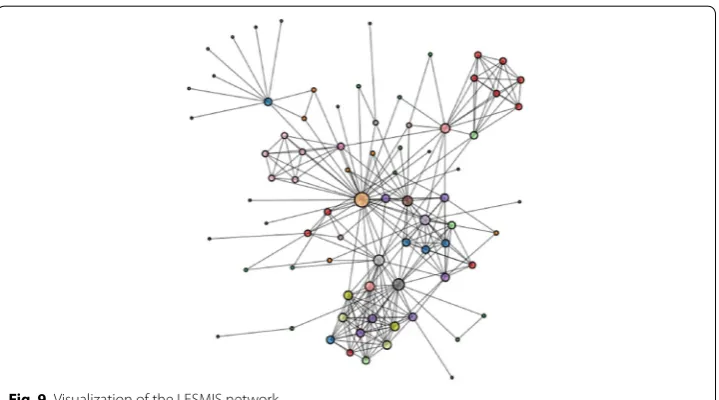
The LESMIS network is patchy at best. This network is included in the collection of Miscellaneous Networks, and describes the coappearance of characters in Les Misera-bles by Victor Hugocontain. The undirected weighted graph contains 77 nodes and 254 edges, and its density is 0.0868079; maximum degree is 36; average degree is 6; assorta-tivity is − 0.165225; number of triangles is 1.4K; average number of triangles is 18; max-imum number of triangles is 82; average clustering coefficient is 0.573137; fraction of closed triangles is 0.498932; lower bound of maximum clique is 10.more information is provide in [26]. As depicted in Fig. 9, visualization of the LESMIS network was obtained via interactive graph visualization platform provided by the networkrepository.com [26].

We obtain a data file in GML format, we convert it into a CSV file. The file con-tains an upper triangular matrix, with all diagonal elements as 0. Note that we have no ground truth about Z and K. For greater reliability, we ran two chains: chain1, which starts with a=b=1,e=24,f =1/HN ; and chain2, which starts with a=b=1,e=44,f =1/HN . We ran each chain for maxIter=10000 MCMC itera-tions, with burnin=4000 and collected the last 6000 samples.

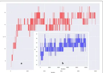
As shown in Fig. 10a, b, both of the two chains show mixing. We illustrate occurring times of all the Ks values sampled from the two chains in Table 4. We can see that for

Fig. 9 Visualization of the LESMIS network

Table 3 Summarization about mode and 95% HPD of retained α ,

chain1 chain2 chain3 chain1 chain2 chain3

Mode of α 2.46 2.75 2.97 95% HPD of α 1.11, 4.47 1.33, 4.78 1.37, 4.94

both of two chains, the mode of all Ks s is 15. Thus, our potential true K value of Go is Ko =15.

From Fig. 11, we can see that the 5962th sample is the last sample drawn from chain1

which satisfied Ks=15 . So, we chose this sample as Z’s posterior inference result, i.e. the observed graph Go ’s community assignment matrix is sampled at the 5962th iteration.

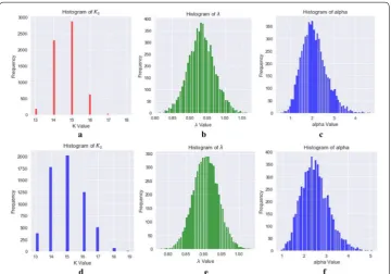
Figure 12 a−c depict the histogram of Ks , α and for the samples retained from chain1, d−f correspond to that of chain2. We can find that although the starting posi-tions of the two chains are different, posterior distribution of the parameters inferred via MCMC are very approximate to each other.

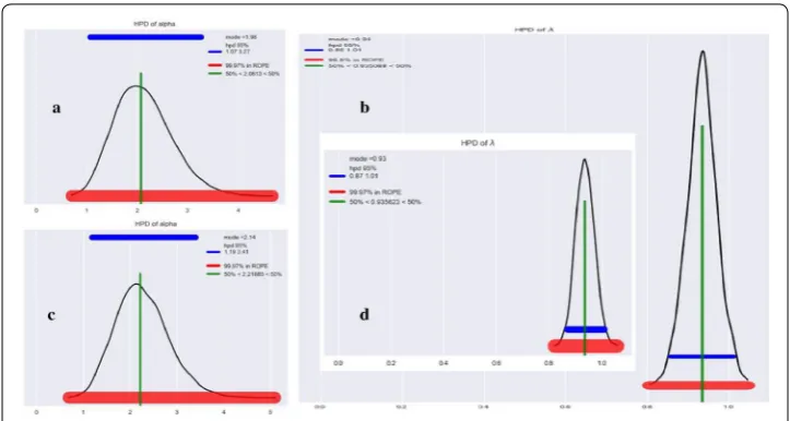
Figure 13a, b depict the HPD of α and for the samples retained from chain1, c−d correspond to that of chain2. We can find that for chain1: the 95% HPD for α is

[1.07, 3.27] and its mode is 1.98; the 95% HPD for is [0.85−1.01] and its mode is 0.94.

For chain2: the 95% HPD for α is [1.19, 3.41] and its mode is 2.14; the 95% HPD for is [0.87−1.01] and its mode is 0.93. From this perspective, the two chains have

approxi-mate inference quality on single variable parameters. But is we compare dispersion of Ks ,

we will find that inference quality of chain1 is better than chain2.

Fig. 10 Trajectory of sampled Ks , a depicted the trajectory of Ks sampled from chain1, b depicted the trajectory of Ks sampled from chain2

Table 4 Occurring times of all the Ks values sampled from the two chains

Ks₌13 Ks₌14 Ks₌15 Ks₌16 Ks₌17 Ks₌18 Ks₌19

Conclusion

The paper makes the following contributions: (1) we propose a generative model for count-value networks with overlapping community structure; (2) we use the IBP to model the community assignment matrix Z, so the number of communities K is not required to be fixed in advance, it is able to increase as more and more data are encoun-tered; (3) both uncollapsed Gibbs sampler and collapsed Gibbs sampler for the gener-ative model have been derived; (4) we analysis the inference quality on single variable parameters; (5) we conduct extensive experiments on simulated network data and real network data, we find that the proposed model and inference procedure can bring us the desired experimental results.

Most count value networks are overdisperse, the negative binomial likelihood is more suitable for these overdisperse count value data. But inference of the rILFM model with negative binomial likelihood requires great care in selecting appropriate starting point, we aim it as one of our future work.

For single variable parameters, the posterior inference result is easy to communicate. But for structured parameters such as Ziks , how to summarize the posterior inference

Fig. 11 Ks value of the last 40 samples drawn from chain1

results and estimate the inference quality, is a considerable challenge, we aim it as another one of our future work.

Abbreviations

rILFM: relational infinite latent feature model; MCMC: Markov chain monte carlo; MMSB: mixed membership stochastic block model; IBP: Indian buffet process; SBM: stochastic block model; IRM: infinite relational model; DCSBM: degree cor-rected SBM; LFRM: latent feature relational model; IMRM: infinite multiple relational; IDCSBM: infinite degree corcor-rected SBM; ILA: infinite latent attribute; HPD: highest posterior eensity; GML: graph model language.

Acknowledgements

We thanks Mikkel N. Schmidt etc. for their great research work and helpful open-source code. Thanks anonymous review-ers for their comments.

Authors’ contributions

QY and ZWY are responsible for model design; QCY and ZW are responsible for model inference; QCY and XFW are responsible for experiment design and experiment implementation; QCY and YZ Wang are responsible for data analysis; QCY, ZW and ZWY are responsible for writing. All authors read and approved the final manuscript.

Funding

This work was partially supported by the National Basic Research Program of China (973) (No. 2015CB352401), the National Natural Science Foundation of China (No. 61332005, 61725205), the Research Project of the North Minzu Uni-versity (No.2019XYZJK02, 2019XYZJK05, 2017KJ24, 2017KJ25, 2019MS002).

Availability of data and materials

Data and materials are online available at https ://githu b.com/yucom puter 2018/rILFM .

Competing interests

The authors declare that they have no competing interests.

Author details

1 _{School of Computer Science and Engineering, Northwestern Polytechnical University, Dongxiang Road, Chang’an} District, Xi’an 710072, China. 2 _{Shanxi Provincial Key Laboratory for embedded system (Northwestern Polytechnical} Uni-versity), Dongxiang Road, Chang’an District, Xi’an 710072, China. 3 _{College of Computer Science, North Minzu University,} YinChuan, China. 4 _{College of Instruments, Jilin University, ChangChun, China.}

Received: 15 May 2019 Accepted: 31 October 2019

References

1. Zhu W, Zhang D, Zhou X, Yang D, Zhiwen Y (2017) Discovering and profiling overlapping communities in location-based social networks. IEEE Trans Syst Man Cybern Syst 44(4):499–509

2. Griffiths T, Ghahramani Z (2005) Infinite latent feature models and the Indian buffet process. In: International confer-ence on neural information processing systems

3. Wang J, Feng W, Wang Y, Zhang D, Qiu Z (2018) Social-network-assisted worker recruitment in mobile crowd sens-ing. IEEE Trans Mob Comput 99:1–1

4. Wang Z, Guo B, Yu Z, Zhou X (2018) Wi-Fi CSI-based behavior recognition: from signals and actions to activities. IEEE Commun Mag 56(5):109–119

5. Airoldi EM, Blei DM, Fienberg SE, Xing EP (2008) Mixed membership stochastic blockmodels. J Mach Learn Res 9(5):1981

6. Erdos P, Renyi A (1959) On random graphs. Publicationes Mathematicae 6(4):3286–3291

7. Brian K, Newman MEJ (2011) Stochastic blockmodels and community structure in networks. Phys Rev E Stat Nonlin-ear Soft Matter Phys 83(2):016107

8. Kemp C, Tenenbaum JB, Griffiths TL (2006) Learning systems of concepts with an infinite relational model. Cogn Sci 21(1):61

9. Karrer B, Newman ME (2011) Stochastic blockmodels and community structure in networks. Phys Rev E Stat Nonlin-ear Soft Matter Phys 83(2):016–107

10. Pensky M (2016) Dynamic network models and graphon estimation. arXiv preprint arXiv :1607.00673 11. Fortunato S (2009) Community detection in graphs. Phys Rep 486(3):75–174

12. Xie J, Kelley S, Szymanski BK (2011) Overlapping community detection in networks: the state-of-the-art and com-parative study. ACM Comput Surv 45(4):1–35

13. Matias C, Robin S (2014) Modeling heterogeneity in random graphs through latent space models: a selective review. ESAIM Proc Surv 47:55–74

14. Miller KT (2011) Bayesian nonparametric latent feature models. Dissertations and Theses—Gradworks, pp 201–226 15. Meeds E, Ghahramani Z, Neal RM, Roweis ST (2006) Modeling dyadic data with binary latent factors. In: International

conference on neural information processing systems

16. Morup M, Schmidt MN, Hansen LK (2011) Infinite multiple membership relational modeling for complex networks. Comput Sci 19(5):1–6

17. Konstantina Palla, Knowles David A, Zoubin Ghahramani (2015) Relational learning and network modelling using infinite latent attribute models. IEEE Trans Pattern Anal Mach Intell 37(2):462–474

18. Herlau T, Schmidt MN, Morup M (2014) Infinite-degree-corrected stochastic block model. Phys Rev E Stat Nonlinear Soft Matter Phys 90(3):032819

19. Aldous David J (1985) Exchangeability and related topics. Springer, Berlin

20. Thibaux R, Jordan MI (2007) Hierarchical beta processes and the Indian buffet process. In: Proceedings of the 11th international conference on artificial intelligence and statistics, pp 1135–1143

21. Zhou M (2015) Infinite edge partition models for overlapping community detection and link prediction. In: In AIST-ATS2015, vol 38, pp 1135–1143

22. De Blasi P, Favaro S, Lijoi A, Mena RH, Prunster I, Ruggiero M (2015) Are gibbs-type priors the most natural generaliza-tion of the dirichlet process? IEEE Trans Pattern Anal Mach Intell 37(2):212–229

23. Doshi F, Miller KT, Van Gael J, Teh YW (2008) Variational inference for the Indian buffet process. J Mach Learn Res 5:137–144

24. Gershman SJ, Blei DM (2012) A tutorial on bayesian nonparametric models. J Math Psychol 56(1):1–12 25. Martin O (2016) Bayesian analysis with python. Packt Publishing

26. Rossi RA, Ahmed NK (2015) The network data repository with interactive graph analytics and visualization. In: Pro-ceedings of the twenty-ninth AAAI conference on artificial intelligence

Publisher’s Note