Pool detection from smart metering data with convolutional neural networks

R E S E A R C H

Open Access

Pool detection from smart metering

data with convolutional neural networks

Cornelia Ferner

, Günther Eibl, Andreas Unterweger, Sebastian Burkhart and Stefan Wegenkittl

FromThe 8th DACH+ Conference on Energy Informatics Salzburg, Austria. 26-27 September, 2019

*Correspondence:

[email protected] Salzburg University of Applied Sciences, Urstein Sued 1, 5412 Puch/Salzburg, Austria

Abstract

The nationwide rollout of smart meters in private households raises privacy concerns: Is it possible to extract privacy-sensitive information from a household’s power

consumption? For a small sample of 869 Upper Austrian households, information about consumption-heavy amenities and household characteristics are available. This work studies the detection of households with swimming pools (the most common amenity in the dataset) using Convolutional Neural Networks (CNNs) applied on load heatmaps constructed from load profiles. Although only a small dataset is available, results show that by using CNNs, privacy can be broken automatically, i.e., without the time-consuming, manual feature generation. The method even slightly outperforms a previous approach that relies on a nearest neighbor classifier with engineered features.

Keywords: Smart metering, Convolutional neural network, Privacy

Introduction

Based on a decision of the European Union, the Austrian Government aims at a 95% coverage for the smart meter rollout in private households until 2022 (RIS - Rechtsin-formationssystem des Bundes2019). Smart meters automatically record the load data in a 15-min interval and, per default, report the numbers once a day. The automated com-munication raises customers’ privacy concerns as knowledge is still sparse about what information can be extracted from 15-min load data (Eibl and Engel2015).

A 2017 survey (Asghar et al. 2017) on smart meter data privacy provides a thor-ough overview of the major concerns related to the collection of load data. Especially, non-intrusive load monitoring (NILM (Hart1992)) could be potentially harmful, as the techniques aim at disaggregating load data to extract load patterns incurred by different devices (Molina-Markham et al.2010; Lisovich and Wicker2018). In addition to detect-ing appliances, previous works by Chen et al. (2013) and Eibl et al. (2018) demonstrate the possibility of detecting the presence or absence of residents, with their work being framed as “occupancy” and “holiday detection”, respectively.

Chen et al. (2016) showed that is possible to locate solar-powered homes based on their energy production signatures, which are location-dependent. For 14 households, they achieved 500-meter accuracy with one-second resolution and 28-kilometer accuracy with one-minute resolution, respectively.

Beckel et al. (2014) showed that demographic data, e.g., the number of residents in a household or whether or not there are children in the household, can be extracted from 30-min load data over a period of one and a half years. They achieved an accuracy of 70% over all 4232 households. For specific characteristics and appliances, the accuracy even exceeded 80%.

Burkhart et al. (2018) investigated a sample dataset of 869 households from Upper Aus-tria (Azarova et al. 2018): In addition to the 15-min load readings, the dataset offers information about whether the household possesses any consumption-heavy amenities, such as a swimming pool, home cinema, aquarium or water bed. By comparing the house-holds’ consumption patterns to the characteristic load profile of a pool filter pump, they were able to correctly detect households with pools with a precision of 68.5% using a nearest neighbor classifier on manually designed features.

This work explores how to automate the pool detection process by training a con-volutional neural network (CNN) (Krizhevsky et al. 2012) directly on the load data. While traditional machine learning methods usually require careful feature generation and selection before applying the classifier, deep learning methods such as the CNN pro-cess the raw data and learn both, how to extract appropriate features and how to classify, at the same time. Thus, no prior knowledge about the domain and data is needed and consequently time and manual effort can be saved.

Since CNNs are usually applied on very large datasets1, it is not known how the method-ology performs for a small dataset like the given one, where only 64 out of 869 households have a pool. The results for pool detection show that the deep learning approach can compete with the approach in (Burkhart et al.2018) that uses manually designed features. While the practical consequences seem marginal, from a privacy perspective the impli-cations are considerable: using CNNs private information can be inferred having both, a small dataset and a small time budget.

This paper is structured as follows: In the Background Section, we provide an overview of the pool detection method from (Burkhart et al.2018) and CNNs. In the Experiments Section, we describe our proposed CNN for automated pool detection and the detection results for the dataset from (Burkhart et al. 2018). In the Discussion and Future Work Section, we compare and discuss these results and provide an outlook to future research directions.

Background

This section describes the existing pool detection method that we use for comparison as well as CNNs that are employed in this work.

Existing pool detection method

Pool detection has already been done in (Burkhart et al. 2018) by exploiting the fact that a swimming pool requires a filter pump. The detection method aims at finding fil-ter pumps which (i) run in a regular manner over the warmest months of the year and (ii) consume several hundred Watts of electrical power, thus constituting a distinct part of the load.

1_{Two famous datasets are MNIST and ImageNet. MNIST (http://yann.lecun.com/exdb/mnist/) is a dataset for}

An important prerequisite for the method is the representation of the time series as a heatmap, where the columns represent days and the rows represent the time of day. Using this representation, the two properties of the pool pump stated above result in more (Fig.1) or less (Fig.2) regular rectangular shapes overlaying the remaining load.

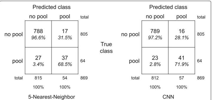
The algorithm detects these rectangular shapes by treating heatmaps as images and by applying image processing methods such as morphological operations. Using a care-fully engineered, sophisticated sequence of steps, the authors achieve a recall of 68% (Fig.4(left)).

Convolutional neural networks (CNN)

Deep neural networks (Goodfellow et al.2016) differ from other machine learning algo-rithms in that they process the raw data directly, i.e., without an explicit feature generation step. The inherent feature generation is one of the big advantages of neural networks, as results can be obtained more quickly without the need for manually engineered features. The raw data passes through the layers of the network which interact in a non-linear fashion.

Feature generation

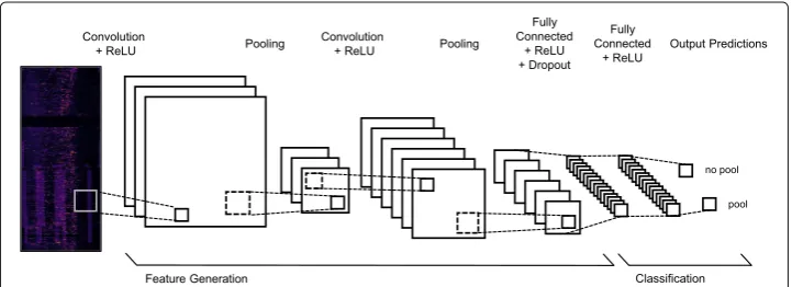
In common network architectures, the first few layers extract features from the given input vectors (4 layers, denoted asFeature Generationin Fig.3). In a convolutional neu-ral network, as described in the following, the first layers are convolutional layers. Each layer consists of a number of filters that detect low level patterns in small spatial regions, e.g., in a 5×5 pixel area2. The output of the convolutional layer passes through the non-linear activation function. The most common activation function is the rectified non-linear unit (ReLU) (Nair and Hinton2010) that assignsf(x)=max(0,x)to each input. The use of ReLU speeds up the training, because the function is easy to compute and to derive. Usually, a pooling layer follows the convolutional layer (see Fig.3). Pooling reduces the feature size in the network and prevents overfitting. The most common form is max pooling which chooses the highest value in a given window (Krizhevsky et al.2012).

Classification

The subsequent classification layers (2 layers, denoted asClassificationin Fig.3), follow a more traditional, dense setup, where each node of one layer is connected with every node of the subsequent layer to learn accurate decision boundaries in the feature space (fully connected). In order to prevent overfitting to the training data, a dropout layer (Srivastava et al.2014) is inserted between two fully connected layers. Dropout means to randomly choose a subset of nodes that is ignored when updating the node weights. The final classification layer, typically a softmax layer (Goodfellow et al.2016), which predicts a vector of probabilities corresponding to the output classes.

Training

The network’s weights are trained by optimizing a loss function based on the error between the network’s predicted output and the target classes. The optimization algorithm iteratively updates the networks’ weights to minimize the classification error. If gradient-based loss optimization is used, the update is commonly known as backpropagation.

Fig. 1Heatmap showing the load [kW] of a household with a pool. This household’s pool pump runs regularly so that the pool features of (Burkhart et al.2018) can be extracted rather easily by detecting the rectangular shaped areas

The trained network weights in the feature generation layers exploit redundant infor-mation in the input data. The output of each layer (activations) represents the discrimi-native information for classification of this input, thus leading to a good, discrimidiscrimi-native representation of the original input.

Experiments

In the following, we present experiments to demonstrate the effectiveness of a CNN to generate suitable features from the input data without any prior knowledge about the problem domain. From a privacy perspective, the intriguing results are disadvantageous: The CNN is a privacy invader. While the development of the method in (Burkhart et al.

Fig. 3 Sketch of the network architecture. The 96x395 heatmaps pass through 4 convolutional layers followed by two fully connected layers. For better visualization, the input data is depicted in color. Note that 4 convolutional layers plus pooling are used instead of the depicted 2

2018) took several weeks, the development of the CNN is much faster, provided that the attacker has suitable skills and tools in both cases.

In order to compare our results to those in (Burkhart et al.2018), we apply our method to the same dataset. It consists of load data (in kW) captured by smart meters with a time granularity of 15 min from 869 households in Upper Austria covering slightly more than one year (396 days). 64 of these households have a swimming pool. As in (Burkhart et al.

2018), each raw time series is converted into a 96×396 heatmap (e.g. Fig.1). In contrast to their approach, we directly pass the heatmaps to the CNN network, so no further feature generation or preprocessing is applied.

Setup of the CNN

The setup loosely follows common basic CNN architectures, especially those of the AlexNet architecture described in (Krizhevsky et al.2012). We set the filter sizes to fit our input image size and to still have sufficiently many nodes left after the feature generation layers. However, as the focus lies on automating the classification process, the parameters and settings have not been further tuned.

More specifically, Fig. 3 displays our network architecture3: We use 4 convolutional layers, each with batch normalization (see below), followed by ReLU and max pooling. The first convolution layers are based on 15 5×5 filters, the subsequent ones use 15 3×3 filters. Filters are moved each time by 1×1 pixels (=stride). At the border, val-ues are computed by extending the image with zeros (padding). The window size of the first pooling layer is chosen to be 5×5 with a stride of 3×3, the latter ones are 3×3 with a stride of 2×2. The pooling layers reduce the feature size from originally 96·396 to 195 (= 15·13, i.e. number of filters · remaining heatmap pixels). The sub-sequent classification layer is a fully connected (dense) layer with 32 nodes with batch normalization and ReLU followed by a 50% dropout layer. The remaining fully connected layer reduces the size to two nodes corresponding to the two classes “pool” and “no pool”. This final layer includes the softmax function producing a distribution over the two classes.

During training, the cross entropy lossL(Goodfellow et al.2016) between the predicted output classyˆand the actual outputyis computed:

L(y,yˆ)= −1 πy

ylog(yˆ)− 1 π1−y(

1−y)log(1− ˆy) (1)

We account for the imbalanced relative amount of heatmaps per class in the dataset (denoted as πy) by applying a weighting inverse to the class distribution to the cross

entropy loss function. This weighting prevents the loss function from overemphasizing on the “no pool” class. Thus, using a binary output with “pool” and “no pool” coded as

y=1 andy=0, respectively.

In order to minimize the loss function, the gradient-based Noam optimizer (Vaswani et al.2017) is used that iteratively updates the weights based on an empirically estimated model sizesand the current epochp. It initially increases the learning rate4rfor a number of warm-up stepswand finally decreases it:

r=s−0.5·minp·w−1.5,p−0.5 (2)

The Noam optimizer is parameterized withw = 15 ands = 1000. The training lasts for 100 epochs, i.e. 100 passes over the training data, and the data is split into batches of size 32. Data batches are used to reduce the input data size. As the network does not see the data at once, we apply batch normalization (Ioffe and Szegedy2015) after each layer to reduce the variance of input values to the next layer.

Results

We evaluate two settings: i) using the CNN as is for classification (CNN pure) and ii) extracting the CNN features (after the fourth convolutional layer) and classifying these features by means of a nearest neighbor classifier (CNN+k-NN). The latter version is intended to study whether the features obtained by the CNN are only suitable within a CNN setting or generalize for different classifiers. In order to compare our results with the ones of (Burkhart et al.2018), the same evaluation methodology is used.

Table1 provides the detailed classification results. As a baseline, we report the clas-sification results from assigning all heatmaps to either the “pool” or the “no pool” class (all-positive and all-negative, respectively). Sin ce the classes are imbalanced, the accu-racy in the all-negative class is already high and therefore, as discussed in (Burkhart et al.

2018), we aim for high precision.

The best classifier with manual features is the 5-nearest neighbors classifier, which achieves 94% accuracy and 68.5% precision (Burkhart et al.2018). When using CNN fea-tures with a k-nearest neighbor classifier, we can maintain the classification accuracy, but lose precision. The best classifier in terms of accuracy only achieves 60.6% of precision. However, the full CNN setting outperforms previous methods and yields 95.5% accuracy and 71.9% precision. Figure4(right) shows the corresponding confusion matrix.

In order to investigate the result more closely, we visually examined the heatmaps of the households with pools to search for the above mentioned rectangular patterns. For some cases, these patterns were not obvious and could only be seen after setting the max-imum load to 2 kW (see Fig.2(bottom)), exploiting the fact that the load of the pump is lower than this value. From the 23 households with an undetected pool, 11 households did not show a rectangular pattern (which is true for only one of the 41 households with a detected pool). One interpretation of this insight is that the 11 households without the

4_{Scaling value which determines to which extent weight values are changed. If the learning rate is too large, the}

Table 1Classification results

Classification Method Accuracy Precision

a) All-positive 10.5% 10.5%

All-negative 89.5%

-b) SVM Gaussian 93.1% 66.7%

5-NN 94.0% 68.5%

1-NN 93.4% 66.7%

c) CNN + 7-NN 93.1% 60.0%

CNN + 5-NN 93.1% 57.7%

CNN + 1-NN 93.4% 60.6%

d) CNN pure 95.5% 71.9%

a) Baseline classification by classifying all instances as “pool” or “no pool”, respectively. b) Classification with manually designed features as in (Burkhart et al.2018). c) Nearest-neighbor classification with CNN features. d) CNN classification

Best performing algorithm in boldface

pattern might not be using their pools, i.e., the pool pump is not running. Households with inactive pools will of course not be detected by any method. Following this interpre-tation, the 11 misclassifications are label errors, not classification errors. Furthermore, the presence of such inactive pools could have the effect of label noise which significantly increases the classification difficulty.

Further experiments with other appliances (home cinema, aquarium) were conducted, but yielded poor results so far. One major issue is the low number of positive samples in the dataset, which is even lower than those of the swimming pools.

Discussion and future work

The results show that convolutional neural networks are able to competitively learn the presence of pools even in the case of a relatively small dataset that contains load profiles of 64 households with pools.

Deep learning is a quickly expanding field with a number of powerful methods to improve the classification process. While pool detection on the given dataset may have reached a limit, as argued above, one could try to predict more rare appliances using data augmentation methods. Generative adversarial networks (GAN) (Goodfellow et al.2014)

are a means to produce artificial, new data but, to the best of our knowledge, have not been applied to time series data (in the form of heatmaps) so far. A siamese network archi-tecture (Koch et al.2015) could be used to train two subnetworks on a pair of heatmaps to decide whether they are from the same class or not. The learned features could be used for classification. The application of a siamese network drastically increases the amount of input data as potentially all 8692image combinations can be used.

From a privacy perspective, the good classification result is negative, since it shows that personal information can be inferred from data in an automatic way, i.e., without manual feature generation, which is typically the most time-consuming modeling step. From this perspective, it is interesting to investigate whether the features learned by the CNN (which showed worse results when combined with k-nearest-neighbor classifier) could reach the performance of the full CNN approach when used with another common classifier.

Similarly, but broadening the scope, it would be interesting to investigate whether the features generalize to other appliances, i.e., whether the features are indicative not only for pools. If so, the features could be used for transfer learning, meaning that the already trained CNN is reused by fixing the weights in the feature layers and only retraining the classification layers on the new task. Moreover, the transfer learning setting could be applied to similar datasets from other countries. A generalization across appliances or countries would have even more negative implications for privacy.

Acknowledgements

The authors would like to thank theEnergieinstitutat the Johannes Kepler University Linz for providing the dataset.

About this supplement

This article has been published as part ofEnergy InformaticsVolume 2 Supplement 1, 2019: Proceedings of the 8th DACH+ Conference on Energy Informatics. The full contents of the supplement are available online athttps:// energyinformatics.springeropen.com/articles/supplements/volume-2-supplement-1.

Authors’ contributions

This paper was written by CF (40%), GE (35%), AU (10%), SB (5%) and SW (10%). The detailed contributions are as follows: The idea for the paper was developed by AU (25%), GE (25%), SW (25%), CF (15%) and SB (10%). The neural network architecture was developed by CF (60%) and SW (40%). The data cleaning was done by SB (90%) and GE (10%). The Abstract was written by CF (50%) and GE (50%). The Introduction section was written by GE (40%), CF (30%) and AU (30%). The Background section on the Existing Pool Detection Method was written by GE (90%) and CF (10%). The Background section on Convolutional Neural Networks was written by CF (50%), SW (30%) and GE (20%). The Experiment section on the setup of the CNN was written by CF (50%), GE (30%) and SW (20%). The Experiment section on the results was written by CF (50%) and GE (50%). The Discussion and Future Work section was written by CF (50%) and GE (50%). All authors read and approved the final manuscript.

Funding

The financial support by the Federal State of Salzburg is gratefully acknowledged. Publication of this supplement was funded by Austrian Federal Ministry for Transport, Innovation and Technology.

Availability of data and materials

For privacy reasons, the data is not publicly available.

Competing interests

The authors declare that they have no competing interests.

References

Asghar MR, Dán G, Miorandi D, Chlamtac I (2017) Smart meter data privacy: A survey. IEEE Commun Surv Tutor 19(4):2820–2835

Azarova V, Engel D, Ferner C, Kollmann A, Reichl J (2018) Exploring the impact of network tariffs on household electricity expenditures using load profiles and socio-economic characteristics. Nat Energy 3:317–325

Beckel C, Sadamori L, Staake T, Santini S (2014) Revealing household characteristics from smart meter data. Energy 78:397–410

Burkhart S, Unterweger A, Eibl G, Engel D (2018) Detecting swimming pools in 15-min load data. In: 2018 17th IEEE International Conference On Trust, Security And Privacy In Computing And Communications/12th IEEE International Conference On Big Data Science And Engineering (TrustCom/BigDataSE). IEEE, New York. pp 1651–1655

Chen D, Barker S, Subbaswamy A, Irwin D, Shenoy P (2013) Non-intrusive occupancy monitoring using smart meters. In: Proceedings of the 5th ACM Workshop on Embedded Systems For Energy-Efficient Buildings. ACM, New York. pp 1–8 Chen D, Iyengar S, Irwin D, Shenoy P (2016) Sunspot: Exposing the location of anonymous solar-powered homes. In:

Proceedings of the 3rd ACM International Conference on Systems for Energy-Efficient Built Environments. BuildSys ’16. ACM, New York. pp 85–94

Eibl G, Burkhart S, Engel D (2018) Unsupervised holiday detection from low-resolution smart metering data. In: ICISSP. SciTePress, Setúbal. pp 477–486

Eibl G, Engel D (2015) Influence of Data Granularity on Smart Meter Privacy. IEEE Trans Smart Grid 6(2):930–939 Goodfellow I, Bengio Y, Courville A (2016) Deep Learning. MIT press, Cambridge

Goodfellow I, Pouget-Abadie J, Mirza M, Xu B, Warde-Farley D, Ozair S, Courville A, Bengio Y (2014) Generative adversarial nets. In: Advances in Neural Information Processing Systems. Curran Associates, Inc., Red Hook. pp 2672–2680 Hart GW (1992) Nonintrusive Appliance Load Monitoring. Proc IEEE 80(12):1870–1891

Ioffe S, Szegedy C (2015) Batch normalization: Accelerating deep network training by reducing internal covariate shift. In: Proceedings of the 32nd International Conference on International Conference on Machine Learning - Volume 37. ICML’15. Microtome Publishing, Brookline. pp 448–456

Koch G, Zemel R, Salakhutdinov R (2015) Siamese neural networks for one-shot image recognition. In: ICML Deep Learning Workshop, vol 2. Microtome Publishing, Brookline

Krizhevsky A, Sutskever I, Hinton GE (2012) Imagenet classification with deep convolutional neural networks. In: Advances in Neural Information Processing Systems. Curran Associates, Inc., Red Hook. pp 1097–1105

Lisovich MA, Wicker SB (2018) Privacy Concerns in Upcoming Residential and Commercial Demand-Response Systems. In: IEEE proceedings on Power Systems, New York. pp 1–10

Molina-Markham A, Shenoy P, Fu K, Cecchet E, Irwin D (2010) Private memoirs of a smart meter. In: Proceedings of the 2nd ACM Workshop on Embedded Sensing Systems for Energy-Efficiency in Building. BuildSys ’10. ACM, New York. pp 61–66

Nair V, Hinton GE (2010) Rectified linear units improve restricted boltzmann machines. In: Proceedings of the 27th International Conference on Machine Learning (ICML-10). Microtome Publishing, Brookline. pp 807–814

RIS - Rechtsinformationssystem des Bundes (2019) Rechtsvorschrift für Intelligente Messgeräte-Einführungsverordnung. https://www.ris.bka.gv.at/GeltendeFassung.wxe?Abfrage=Bundesnormen&Gesetzesnummer=20007808. Accessed 4 May 2019

Srivastava N, Hinton G, Krizhevsky A, Sutskever I, Salakhutdinov R (2014) Dropout: A simple way to prevent neural networks from overfitting. J Mach Learn Res 15:1929–1958

Vaswani A, Shazeer N, Parmar N, Uszkoreit J, Jones L, Gomez AN, Kaiser Ł., Polosukhin I (2017) Attention is all you need. In: Advances in Neural Information Processing Systems. Curran Associates, Inc., Red Hook. pp 5998–6008

Publisher’s Note

Springer Nature remains neutral with regard to jurisdictional claims in published maps and institutional affiliations.

Submit your manuscript to a

journal and benefi t from:

7Convenient online submission

7Rigorous peer review

7Immediate publication on acceptance

7Open access: articles freely available online

7High visibility within the fi eld

7Retaining the copyright to your article