Global structural changes and their implication for territorial CO2 emissions

Global structural changes and their

implication for territorial CO

₂

emissions

K. Shironitta

1 Background

Global territorial GHG emissions have increased continuously as nations have pursued economic growth. The average annual increase in GHG emissions for the decade 2000 through 2010 is 2.2 % (IPCC 2014). According to Assessment Report 5 of the Intergov-ernmental Panel for Climate Change (IPCC), CO2 remains the major GHG, account-ing for 76 % of total GHG emissions. Changes in human population, per-capita gross domestic product (GDP), energy intensity of production, and CO2 emission intensities of energy production have affected fossil fuel-related CO2 emissions by +87, +103, −35, and −15 %, respectively, over the 40-year period from 1970 to 2010 (IPCC 2014). These data imply that the positive effects of energy efficiency improvements on CO2 emissions have been canceled out by the increase in per-capita production and population.

While territorial and consumption-based CO2 emissions in Asia increased at relatively comparable rates from 1990 to 2010 (i.e., 175 and 197 %, respectively), consumption-based CO2 emissions in the OECD member nations increased at least three times as quickly as territorial CO2 emissions (i.e., production-based CO2 emissions) over the

Abstract

This paper proposes a comprehensive decomposition method to estimate how changes in domestic economic scale, industrial composition, domestic technology, export scale of intermediate products, export composition of intermediate products, export scale of final products, export composition of final products, import scale of intermediate products, import composition of intermediate products, import scale of final products, import composition of final products, and foreign technology affect the volumes of both territorial CO2 emissions (including emissions induced by producing exports) and extraterritorial CO2 emissions induced by imports. Specifically, the sources of the territorial CO2 emissions of each of 40 nations from 1995 to 2009 were examined using the Environmentally Extended World Input–Output Tables in 2009 prices. Based on the results, the patterns of structural change in the 40 nations can be classified into eight types and it can be seen that domestic industrial structure changes and import structure changes have different roles according to the group types. This study dem-onstrates the need for global warming countermeasures that consider the differences in the role that each country’s structural changes play in CO2 emissions. We also found that the export composition effect was negligibly small in both the high-income and middle-income group of countries during 1995–2008 and it has not played an impor-tant role in climate change.

Open Access

© 2016 The Author(s). This article is distributed under the terms of the Creative Commons Attribution 4.0 International License (http://creativecommons.org/licenses/by/4.0/), which permits unrestricted use, distribution, and reproduction in any medium, provided you give appropriate credit to the original author(s) and the source, provide a link to the Creative Commons license, and indicate if changes were made.

RESEARCH

same period (IPCC 2014). The reason for this remarkable increase in consumption-based CO2 emissions in OECD member nations has been the growing dependence on Asia for imports, which implies that the increase in CO2 emissions was attributable to international trade (Hertwich and Peters 2009; Davis et al. 2011; Peters et al. 2011).

Compared to territorial CO2 emissions, however, the accounting method for con-sumption-based CO2 emissions poses additional challenges, including the requirement for a deeper understanding of the global supply chain complexity associated with the final demand of nations. Conversely, accounting for the CO2 emissions directly gener-ated to produce products (i.e., production-based CO2 emissions) is relatively straight-forward. Therefore, it would be useful to be able to estimate the production-based CO2 emissions responsible for exports when evaluating how importing countries contribute directly to CO2 emissions induced by the domestic production activities of exporting countries. It is crucial to monitor the driving forces of the changes in not only produc-tion-based emissions but export-based emissions in making a climate change policy with a focus of territorial emissions.

In this study, we focus on recent changes in domestic economic structure in the world. The World Input–Output Database (WIOD) covering 40 developed and developing countries shows that from 1995 to 2009, the ratio of domestic output in the tertiary sec-tors of the 40 countries to the total output of those countries grew by 1.1 %, whereas that of domestic production in the primary and secondary sectors of those countries declined by 4.4  % (Dietzenbacher et  al. 2013). In addition, the dependence of the 40 countries on imports of primary and secondary products during the same period grew at rates of 2.1 %. In other words, domestic industrialization has rapidly weakened from 1995 to 2009 and this structural change has affected the environment.

and so did not include empirical decomposition results that took into account produc-tion-based emissions, which should also be discussed by climate policy makers.

This paper proposes an additive decomposition method of production-based emis-sions and empirically examines the extent to which changes in the global industrial structure as well as changes in import structure and export structure have contributed to changes in production-based CO2 emissions (i.e., territorial CO2 emissions). Spe-cifically, the territorial CO2 emissions of each of the 40 aforementioned nations from 1995 to 2009 were estimated using the Environmentally Extended World Input–Output Tables at 2009 prices (Dietzenbacher et al. 2013; Timmer et al. 2015). The Shapley–Sun– Dietzenbacher–Los additive decomposition method (Park 1992; Dietzenbacher and Los 1997, 1998; Sun 1998; Ang et al. 2003; Ang 2004; Nansai et al. 2007, 2009; Kagawa et al. 2012) was then applied to examine the sources of changes in the territorial CO2 emis-sions. Based on these results, we examine how these structural changes have contributed to changes in CO2 emissions. It should be noted that empirical results from the addi-tive decomposition used in this study are not directly comparable to those from previ-ous studies using multiplicative decomposition techniques (e.g., Voigt et al. 2013; Xu and Dietzenbacher 2014).

The remainder of this paper is organized as follows: Sect. 2 describes the study meth-odology, Sect. 3 presents the data, Sect. 4 gives results and discussion, and Sect. 5 con-cludes the paper.

2 Methods

In this study, we clarify how a widely used multiregional input–output database is useful for estimating the effects of changes in industrial composition and trade patterns on pro-duction-based emissions. We employ additive decomposition techniques to examine the effects of technology, industrial composition, and economic scale on production-based emissions (Park 1992; Sun 1998; Ang et al. 2003; Ang 2004). Furthermore, we develop a decomposition method for examining the effects of changes in the composition of both regional and sectoral imports on CO2 emissions.

The WIOD database from 1995 to 2009 (Dietzenbacher et al. 2013; Timmer et al. 2015) covers 35 industrial sectors and 40 countries (Tables 4, 5 in the Appendix). Using the time series multiregional input–output tables, total territorial emissions Qt_d(s) induced by manufacturing activities in country s in year t can be expressed as follows:

where et_(s)=et

i(s)

, θt_(s)=θt

i(s)

, and X_dt(s) are the emission intensity row vector describing CO2 emissions per unit output in industrial sector i in country s in year t, the industrial composition column vector describing the fraction of output from industry sector i of total production across all industries in country s in year t, and total industrial output summed over all industrial sectors in country s in year t, respectively. The sub-script d denotes “domestic.” N is the number of industrial sectors.

The annual change in Qt_d(s) from year t to year t ₊ 1 is then

(1)

Q_dt(s)= N

i=1

et_i(s)θ_it(s)X_dt(s)

which can be re-arranged as

The first term on the right-hand side of Eq. (3) represents the effects of changes in CO2 emission intensities on the estimated CO2 emissions, and the second and third terms represent the influence of changes in industrial composition and in gross output on CO2 emissions, respectively; the remaining four terms are interaction terms. Using the Shap-ley–Sun–Dietzenbacher–Los decomposition to classify the seven terms (including the interaction terms among the technology effect, the industrial composition effect, and the economic scale effect), the following is obtained:

For notational convenience, the symbol s denoting country is omitted.

Equation (4) does not allow an examination of the sources of changes in extraterri-torial emissions due to direct imports of intermediate products that are necessary for domestic production and direct imports of final products. Therefore, in this study, the emissions associated with the direct imports of intermediate products and final prod-ucts are formulated as follows:

where Qt_m(s), λt,r_(s)=λt,rs i (s)

, πt,r_(s)=πt,rs

i (s)

, IMt_z(s), and M_ft(s) are the total territorial emissions caused by imports, the import composition column vectors of the ratios of imports by industrial sector i into country s to the total imports for intermedi-ate products and final products to country s, the total amount of imports of intermediate

(2) �Qd(s)=et+1(s)θt+1(s)Xdt+1(s)−et(s)θt(s)Xdt(s)

(3) �Qd(s)=�e(s)θt(s)Xdt(s)+et(s)�θ(s)Xdt(s)+et(s)θt(s)�Xd(s)

+�e_(s)�θ_(s)Xt

d(s)+et(s)�θ(s)�Xd(s)+�e(s)θt(s)�Xd(s)

+�e_(s)�θ_(s)�Xd(s)

(4) Qd=eθtXdt+

1 2

eθ_Xt

d+eθtXd

+1

3eθXd

Technology effect

+etθ_Xt

d+ 1 2

eθ_Xt

d+etθXd+ 1 3

eθ_Xd

Industrial composition effect

+etθt_Xd+1

2

eθt_X

d+etθXd

+1

3

eθ_Xd

Economic scale effect

(5)

Q_mt(s)=

R

r=1,r�=s N

i=1

et_i(r)λt_i,rs(s)IM_zt(s)+

R

r=1,r�=s N

i=1

et_i(r)π_it,rs(s)IM_ft(s)

=

R

r=1,r�=s

et_(r)λt,r_(s)IMt

z(s)+ R

r=1,r�=s

et_(r)πt,r_(s)IMt

products, and the total amount of imports of final products for country s, respectively.

et_(r)=et

i(r)

is the emission intensity row vector for country r, and R is the number of countries.

The extraterritorial emissions due to importation can be decomposed in the same way, i.e., into the effects of technology, domestic import structure, and domestic import scale in the importing country:

The emissions associated with the direct export of intermediate products and final products are formulated as follows:

where Qt_x(s), εt,r_(s)=εt,sr i (s)

, δt,r_(s)=δt,sr i (s)

, EX_zt(s), and EX_ft(s) are the total territorial emissions caused by exports, the export composition column vectors of the ratios of exports by industrial sector i from country s to the total exports of intermedi-ate products and final products to country r, the total amount of exports of intermediate products, and the total amount of imports of final products for country r, respectively.

et_(s)=et

i(s)

is the emission intensity row vector for country s.

Territorial CO2 emissions due to exportation can be decomposed into the effects of technology, domestic export structure, and domestic export scale in the exporting country:

(6) Qm=eλt_IMt

z+ 1 2

eλ_IMt

z+eλtIMzt

+ 1

3eλIMz

Overseas technology effect for intermedaite products

+eπt_IMt

f + 1 2

eπ_IMt

f +eπtIMf

+ 1

3

eπ_IMf

Overseas technology effect for final products

+etλ_IMt

z+ 1 2

eλ_IMt

z+etλIMz

+ 1

3eλIMz

Import composition effect for intermedaite products

+etλ_IMt

z+ 1 2

eπ_IMt

f +etπIMf

+1

3eπIMf

Import composition effect for final products

+etλt_Mz+1

2

eλt_IMz+etλ_IMz+ 1

3eλIMz

Import scale effect for intermedaite products

+etπt_IMf +1

2

eπt_IMf +etπ_IMf+ 1

3

eπ_IMf

Import scale effect for final products

(7) Q_xt(s)=

R

r=1,r�=s N

i=1

et_i(s)ε_it,sr(s)EX_zt(s)+

R

r=1,r�=s N

i=1

et_i(s)δ_it,sr(s)EX_ft(s)

=

R

r=1,r�=s

et_(s)εt,r_(s)EXt

z(s)+ R

r=1,r�=s

et_(s)δt,r_(s)EXt

3 Data

In this study, the WIOD (Dietzenbacher et al. 2013; Timmer et al. 2015) and the Environ-mental Accounts, which are downloadable from the data website: http://www.wiod.org/ new_site/data.htm, are employed. These data cover 35 industrial sectors and 40 coun-tries and region (Tables 4, 5 in the Appendix) and focus on the period of 1995–2011. For this study, the nominal World Input–Output Tables for 1995–2009 were converted into deflated World Input–Output Tables based on 2009 prices using the double deflation method (United Nations 1999). The deflators were obtained from the output prices of the nominal World Input–Output Tables and of the real World Input–Output Tables in previous year’s prices.

The industrial composition column vector and total industrial output of 40 countries and region are calculable from the domestic outputs described in the deflated World Input–Output Tables, and the industrial CO2 emissions for 40 countries are obtainable from the Environmental Accounts (Dietzenbacher et al. 2013; Timmer et al. 2015). The emission intensity row vector can be easily obtained by dividing industrial CO2 emis-sions by industrial outputs. The data on intermediate inputs and final demand of goods and services are directly obtainable from the deflated World Input–Output Tables.

4 Results and discussion

In this section, the results of year-on-year changes in territorial CO2 emissions in 40 countries over the 15-year period from 1995 to 2009 are described using the decom-position method formulated in the previous section. Per-capita incomes published by the World Bank for the 40 countries (World Bank 2013) were used to classify the coun-tries into three groups: high-income nations with per-inhabitant annual incomes of ≥$12,616, middle-income nations with per-inhabitant annual incomes of ≥$4086 and <$12,616, and low-income nations with per-inhabitant annual incomes of <$4086. For (8) Qx=eεtEXzt+

1 2

eε_EXt

z+eεtEXz+ 1

3eεEXz

Domestic technology effect for intermedaite products

+eδt_EXt

f + 1 2

eδ_EXt

f +eδtEXf

+ 1

3eδEXf

Domestic technology effect for final products

+etε_EXt

z+ 1 2

eε_EXt

z+etεEXz+ 1

3eεEXz

Export composition effect for intermedaite products

+etδ_EXt

z+ 1 2

eδ_EXt

f +etδEXf

+ 1

3eδEXf

Export composition effect for final products

+etεt_EXz+1

2

eεt_EXt

z+etεEXz+ 1

3eεEXz

Export scale effect for intermedaite products

+etδt_EXf +1

2

eδt_EXt

f +etδEXf

+ 1

3

eδ_EXf

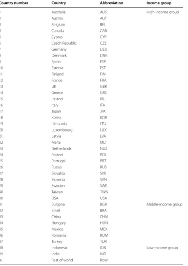
this study, 31 of the 40 countries were classified as high-income, seven were classified as middle-income, and two were classified as low-income (Tables 5 in the Appendix).

4.1 Economic scale effect, industrial composition effect, and domestic technology effect This study focused on four periods (1995–2000, 2000–2005, 2005–2008, and 2008– 2009) and estimated the effects of changes in economic scale, industrial composition, and domestic technology during those periods using Eq. (4). Table 1 shows the decom-position results on “country average” in the three groups. It should be noted that the international financial crisis occurred between 2008 and 2009.

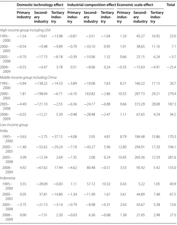
Table 1 Results of decomposing territorial CO₂ emissions (Unit: Mt CO₂)

Domestic technology effect Industrial composition effect Economic scale effect Total Primary

industry Second-ary industry

Tertiary indus-try

Primary indus-try

Second-ary industry

Tertiary indus-try

Primary indus-try

Second-ary industry

Tertiary indus-try

High-income group including USA 1995–

2000 −1.54 −19.61 −13.98 −0.87 −3.51 −1.04 1.33 45.27 16.92 23.0 2000–

2005 −0.54 −0.48 −9.89 −0.70 −33.10 0.95 1.01 38.65 11.16 7.1 2005–

2008 −0.70 −17.73 −8.18 −0.39 −10.06 1.32 0.66 25.15 6.24 −3.7 2008–

2009 −0.55 −0.47 3.78 0.51 −8.06 0.24 −0.35 −15.63 −4.91 −25.4 Middle-income group including China

1995–

2000 −5.84 −138.22 −14.53 −3.89 −10.06 7.63 8.21 166.22 17.15 26.7 2000–

2005 1.81 −198.04 −6.71 −6.10 163.82 −2.86 10.55 287.73 29.21 279.4 2005–

2008 −4.49 −121.10 −2.55 −6.56 −24.17 −6.88 9.66 315.29 28.08 187.3 2008–

2009 −0.55 −12.21 5.39 −0.48 −28.48 −2.47 1.11 67.65 4.24 34.2 Low-income group

India 1995–

2000 −3.63 −2.75 −37.15 −4.08 3.95 4.81 8.79 184.48 15.86 170.3 2000–

2005 −1.40 −55.62 −29.24 −7.19 −43.27 5.96 12.80 294.91 17.20 194.1 2005–

2008 3.99 −12.34 2.69 −7.35 2.06 0.24 10.45 269.26 12.59 281.6 2008–

2009 4.92 −67.62 17.94 −4.62 80.48 −0.51 3.53 95.42 5.42 135.0 Indonesia

1995–

2000 3.55 −28.09 −0.83 1.11 57.12 10.32 0.43 5.22 1.05 49.9 2000–

2005 0.05 37.81 −14.80 −1.34 −11.90 1.67 3.61 44.89 7.48 67.5 2005–

2008 −3.75 −21.13 −3.14 −0.79 −8.98 −0.31 2.63 43.67 5.38 13.6 2008–

The economic scale effect reflects the influence of changes in the overall domestic industrial output on CO2 emissions. The cumulative economic scale effect in the high-income nations contributed to an increase in emissions of 146 Mt CO2 in the three industries from 1995 to 2008 (Table 1). On the other hand, territorial CO2 emissions decreased by 21 Mt CO2 in the three industries in response to the economic recession that followed the international financial crisis between 2008 and 2009 (see the eco-nomic scale effect in the high-income nation group during the 2008–2009 period in Table 1). Interestingly, during the 2008–2009 period, when the effect of the financial cri-sis reduced the average output of the high-income nations by 5.9 %, CO2 emissions in the high-income nations also decreased by 5.4 %. In other words, the economic damage resulting from the financial crisis was partially offset by social benefits from a reduc-tion in CO2 emissions. Prior to 2005, the cumulative effect of output growth in the high-income nations amounted to approximately 50–60 Mt CO2 every 5 years.

Conversely, the cumulative economic scale effect in the middle-income nations, such as China and Turkey, was 872 Mt CO2, which is six times that of the high-income nations from 1995 to 2008 (see the economic scale effect in the middle-income nations of Table 1). The growth in the economic scale effect of the middle-income nations in each of the three periods was extremely high at 192 Mt CO2 in 1995–2000, 328 Mt CO2 in 2000–2005, and 353 Mt CO2 in 2005–2008 (Table 1). Indeed, the rapid economic growth of the middle-income nations is the source of much of the world’s CO2 emissions increases. Examin-ing the sectoral breakdown of industries as they relate to the mean cumulative economic scale effect in the middle-income nations, we find that primary industries contributed 28 Mt CO2, secondary industries contributed 769 Mt CO2, and tertiary industries contrib-uted 74 Mt CO2 of CO2 emissions from 1995 to 2008 (see Table 1; Table 4 in the Appendix for industry groups). The growth of secondary industries in the middle-income nations therefore brought about an abrupt increase in CO2 emissions. Importantly, compared to the high-income nations, the economic scale effect in the middle-income nations during the financial crisis was positive, and consequently, even in the financial crisis, CO2 emis-sions in the middle-income nations (especially in China) have increased faster than the decrease in CO2 emissions in the high-income nations.

The industrial composition effects illustrate how changes in domestic industrial com-position influence CO2 emissions. The cumulative industrial composition effect per country in the high-income nations was −47 Mt CO2, a reduction in CO2 emissions in the three industries from 1995 to 2008 (Table 1). Breaking down the composition of the industries and their CO2 emissions, we find that primary industries contributed −2 Mt CO2, secondary industries contributed −47 Mt CO2, and tertiary industries contrib-uted 1 Mt CO2 during the study period (Table 1). In addition, the industrial composition effect of secondary industries took on a large negative value because the emission inten-sities of secondary products are relatively high. On the other hand, the industrial com-position effect of tertiary industries was close to neutral on CO2 emissions. Thus, it is clear that the changes in the industrial composition of the high-income nations, namely the shift away from manufacturing to services, have contributed to reducing the territo-rial CO2 emissions of that group.

middle-income nations increased domestic CO2 emissions (see the third column of Table 1). Similarly, from the calculated breakdown by industry, primary industries con-tributed −17 Mt CO2, secondary industries contributed +130 Mt CO2, and tertiary industries contributed −2 Mt CO2 (Table 1). In contrast to the high-income nations, the middle-income nations heavily industrialized, and the resulting increase in emis-sions (+111 Mt CO2) due to industrialization in the middle-income nations exceeded the reduction in emissions (−47 Mt CO2) due to deindustrialization of the high-income nations. Ultimately, changes in industrial activities in both income groups contributed to global warming.

Production technologies have played a crucial role in global warming (IPCC 2014). Therefore, we also examined the extent to which changes in emission intensities due to changes in domestic technologies influenced CO2 emissions. The cumulative domestic technology effect in the high-income nations in the three industries from 1995 to 2008 was −73 Mt CO2 per country (Table 1); this decrease is considered to reflect efforts by the high-income nations to adopt environmentally benign production activities. The sec-ondary and tertiary industries showed particularly high cumulative technology effects, at −38Mt CO2 and −32 Mt CO2, respectively, per country from 1995 to 2008 (Table 1). During the same period, domestic technology effects in the middle-income nations (e.g., China and Turkey) accounted for −490 Mt CO2 per country, which was approxi-mately seven times the cumulative domestic technology effect of the high-income nations. Compared to the high-income nations, which are relatively more technologi-cally advanced, the middle-income nations have more room for technological develop-ment; as they make further advances in the future, they will have considerable potential to reduce emissions.

4.2 Export scale effect and export composition effect

time, in developing economies such as those of the middle-income group of countries, it is necessary to implement emission control measures that are focused on the volumes of manufactured exports.

4.3 Import scale effect, import composition effect, and foreign technology effect

Concomitant with the shift of domestic economies away from manufacturing to ser-vices has come an increasing dependence on the importation of manufactured goods, which has increased the emissions associated with imports (in this study, this increase in imports was observed to have the effect of increasing the territorial CO2 emitted in the import-partner country during production of goods for export). The emissions induced by imports consist of the territorial emissions associated with the production of the intermediate and final imported products. According to the data in the WIOD (Dietzen-bacher et al. 2013), the import interdependence among the high-income nations in the 1995–2009 period decreased to approximately 10 %, while the fraction of imports in the high-income nations from the middle- and low-income nations almost doubled. Thus, the import dependence on developing countries is increasing rapidly, and these changes in the import structures of developed nations have accelerated CO2 emissions in devel-oping nations.

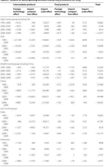
Table 2 shows how the extraterritorial emissions attributed to imports can be decom-posed into the import scale effect, import composition effect, and the foreign technology effect estimated by Eq. (6). The import scale effects for intermediate and final products shown in Table 2 are the effects of changes in total domestic imports on emissions in the import-partner country. Imports by the high-income nations decreased markedly due to the international financial crisis, resulting in the import scale effect being negative from 2008 to 2009 (see Table 2). In the high-income group, the cumulative import scale effects associated with the production of intermediate and final products were 27 Mt CO2 and 6 Mt CO2 per country, respectively, during the 1995–2008 period.

In the middle-income nations, the cumulative import scale effects associated with the production of imports of intermediate and final products were 53 Mt CO2 and 10 Mt CO2, respectively, during the 1995–2008 period. The import scale effect in the middle-income nations was greater than that in the high-middle-income nations; in particular, the effect due to imports of intermediate products was twice that in the high-income nations (see Table 2). The main reason for this was that during the shift away from manufacturing by the high-income nations, although the demand for imports of intermediate prod-ucts from secondary industries decreased, the demand for the same secondary indus-try products increased in the middle-income nations due to increased industrialization capacity and foreign trade.

Table 2 Results of decomposing extraterritorial CO2 emissions (Kt CO2)

Intermediate products Final products Total

Foreign technology effect

Import composi-tion effect

Import

scale effect Foreign technology effect

Import composi-tion effect

Import scale effect

High-income group including USA

1995–2000 −4122 708 12,622 −492 38 2127 10,882

2000–2005 −3015 783 6920 −856 283 2033 6148

2005–2008 −2536 −1602 7088 −685 −87 1441 3619

2008–2009 −1490 −795 −8989 −813 −68 −322 −12,477 USA

1995–

2000 −27,169 21,424 118,882 −359 −2263 6600 117,116 2000–

2005 −19,536 −7165 42,902 −2922 −1220 2640 14,698 2005–

2008 −18,629 −438 14,978 −2055 −774 2565 −4354 2008–

2009 −5504 −25,666 −56,293 −1754 553 254 −88,410 Middle-income group including China

1995–2000 −445 −342 11,714 −491 −1723 4008 12,034 2000–2005 −2715 −1848 16,776 −47 −565 3712 15,425 2005–2008 −1305 −3191 24,823 −1186 −1292 2335 17,791 2008–2009 −2471 1474 −7146 −1211 −347 317 −8608 China

1995–

2000 978 204 35,284 1315 −2278 3335 37,660

2000–

2005 −9009 −11,775 94,489 1824 −656 3864 95,604 2005–

2008 −5420 −20,892 138,921 −901 −1821 855 99,488 2008–

2009 −8881 15,244 −21,549 −752 609 443 −18,692 Low-income group

India 1995–

2000 −2634 −3697 15,998 −783 −60 1778 10,602

2000–

2005 486 23,733 20,817 228 1103 1421 47,787

2005–

2008 −1227 −9402 14,751 −282 −536 1273 4578

2008–

2009 −12,201 −169 −4587 1448 −93 −578 −16,179 Indonesia

1995–

2000 −1150 289 3169 −706 885 −398 9998

2000–

2005 54 1580 4298 −517 854 217 7802

2005–

2008 91 −1302 5162 −476 2 533 −3147

2008–

composition effects (Table 2) for each income group shows that in the 10 years between 1995 and 2005, changes in the industrial composition of the high-income nations helped to reduce CO2 emissions, but changes in import patterns as a result of factors such as import substitution caused CO2 emissions to increase. Interestingly, in the three years from 2005 to 2008, changes in the import patterns of intermediate products by the high-income nations mitigated global warming.

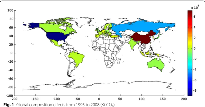
Figure 1 is a world map showing the net industrial composition effect (that is, the industrial composition effect plus the import composition effect) of 40 countries from 1995 to 2008. The figure shows to what degree a nation’s industrial structure (also tak-ing import structure into account) contributes to increastak-ing or decreastak-ing emissions. As shown, China and the USA have very large net industrial composition effects. While changes in its industrial structure enabled the USA to achieve an 895 Mt CO2 reduc-tion in emissions, changes in the industrial structure of China resulted in a 720 Mt CO2 increase in emissions. As in Tian et  al. (2014), for the study period (1995–2008), we found that the industrial composition change in the four heavy manufacturing sectors of Basic Metals and Fabricated Metal, Machinery, Electrical and Optical Equipment, and Transport Equipment in China led to a rapid increase in CO2 emissions amounting to 17 % of the effect of the China’s structural changes (119 Mt CO2). Compared to these two major countries, changes in the industrial structure of European nations have had almost no impact on CO2 emissions. These data show that these two major countries will have major roles regarding CO2 emissions forward into the future.

4.4 Discussion

Since the import composition effect of intermediate products and final products in Table 2 can be estimated from the third and fourth terms, respectively, on the right-hand side of Eq. (6), larger intermediate and final product imports of a country imply a greater import composition effect. To grasp the impact that pure import pattern changes have on CO2 emissions, the ‘normalized’ import composition effect was estimated by divid-ing the import composition effect of intermediate products and that of final products by their respective import values. Similarly, the larger a country’s domestic output value is,

the greater its industrial composition effect will be; thus, a “normalized” industrial com-position effect was estimated by dividing the industrial comcom-position effect by the domes-tic output. By comparing the estimated normalized import composition effect and the normalized industrial composition effect for each country, it is possible to analyze the role that each country’s pure structural changes play in global warming.

Table 3 shows the normalized import composition effect and normalized industrial composition effect for intermediate and final products in the 40 countries examined in this study. Based on the estimation results, the patterns of structural change in the 40 nations can be classified into eight types. The largest type group is Type II, which com-prises nations for which the normalized industrial composition effect and normalized import composition effect for intermediate products are both negative, but normalized import composition effect for final products is positive. Type II countries, which include Japan, the UK, and Mexico, have reduced their emissions through structural changes (e.g., transitioning to a service economy), but have increased their emissions indirectly by increasing their import composition of emissions-intensive products for final prod-ucts. The net composition effects (i.e., the sum of the normalized import composition effect for intermediate products, the normalized import composition effect for final prod-ucts, and the normalized industrial composition effect) for most of countries of Type II are negative, which implies that their structural changes are environmentally good in the sense that they reduced emissions. However, the normalized import composition effects of final products for Japan, Luxembourg, and Mexico are relatively large compared to other countries classified as Type II, which resulted in positive net composition effects. This was especially high for Japan, which had the largest normalized import composi-tion effect of final products among the high-income nacomposi-tions, and its structural changes, including its import structure changes, have contributed to increasing its CO2 emissions.

Interestingly, the net composition effect is very high (2.805; the total shown in Table 3) in Bulgaria (Type V), which was industrializing more rapidly than other countries between 1995 and 2008. Despite significant structural changes in Bulgaria, the com-position effects of both intermediate product imports and final product imports were negative and these import activities contributed greatly to mitigate its responsibility for global warming. At 2.219, Indonesia (Type VIII) had the second highest net composition effect, but that is still markedly different from Bulgaria. Domestic structural changes in Indonesia have also caused emissions to increase, as in Bulgaria, but in Indonesia changes in import patterns have also contributed to global warming. Indonesia should therefore try to mitigate its contribution to global warming by encouraging the impor-tation of substitutes for products that cause significant emissions. As for Bulgaria, it underwent its emissions-intensive industrial structural change relatively early compared to other countries and therefore should adopt policies aimed at reducing emissions from emissions-intensive industries. Thus, the impacts that structural changes have on CO2 emissions vary and are independent of a nation’s level of development.

For example, in countries belonging to Type II, changes in import structure of final prod-ucts contribute to global warming, and therefore mitigation countermeasures should be focused on shifting emissions-intensive technologies of final products produced over-seas and/or trade patterns of final products. In countries belonging to Type IV or VIII, Table 3 Effects of industrial and import composition changes on CO2 emissions

Country Income

group Normalized import com-position effect of immediate products

Normal- ized import composition effect of final products

Normalized industrial composition effect

Total Type

for structural changes

EST High −0.079 −0.075 −0.577 −0.731 Type I

FIN High −0.125 −0.020 −0.045 −0.189

ITA High −0.119 −2.319 −0.009 −2.446

SVK High −0.181 −0.017 −0.037 −0.234

CZE High −0.097 0.020 −0.158 −0.236 Type II

GBR High −0.076 0.076 −0.059 −0.058

HUN Middle −0.173 0.065 −0.130 −0.238

JPA High −0.474 0.955 −0.098 0.383

LUX High −0.078 0.202 −0.016 0.108

LVA High −0.145 0.100 −0.030 −0.074

MEX Middle −0.002 0.102 −0.010 0.090

POL High −0.072 0.016 −0.102 −0.158

ROM High −0.087 0.004 −0.209 −0.292

RUS High −0.145 0.001 −0.411 −0.554

BEL Middle 0.399 −0.155 −0.039 0.206 Type III

BRA Middle 0.028 −0.114 −0.007 −0.094

CAN High 0.103 −0.091 −0.022 −0.010

KOR High 0.040 −0.712 −0.006 −0.678

SVN High 0.143 −0.051 −0.038 0.054

SWE High 0.048 −0.007 −0.019 0.022

USA High 0.034 −0.108 −0.120 −0.194

AUS High 0.033 0.047 −0.091 −0.011 Type IV

IND Low 0.083 0.016 −0.033 0.066

LTU High 0.039 0.603 −0.066 0.577

NLD High 0.099 0.029 −0.031 0.097

BGR Middle −0.109 −0.152 3.066 2.805 Type V

CHN Middle −0.030 −0.136 0.072 −0.095

FRA High −0.041 −0.219 0.001 −0.259

TWN High −0.123 −0.029 0.254 0.102

CYP High −0.121 0.419 0.146 0.444 Type VI

ESP High −0.031 0.002 0.031 0.003

PRT High −0.012 0.161 0.124 0.273

AUT High 0.042 −0.240 0.016 −0.182 Type VII

DEU High 0.029 −0.010 0.026 0.046

TUR Middle 0.053 −0.104 0.063 0.012

DNK High 0.028 0.042 0.066 0.137 Type VIII

GRC High 0.067 0.267 0.054 0.387

IDN Low 0.016 2.066 0.137 2.219

IRL High 0.003 0.080 0.012 0.095

changes in import structure contribute to global warming; consequently, mitigation countermeasures adopted by these countries need to focus on trade patterns. On the other hand, in countries of Types V to VIII, industrial structure change contributes to global warming and therefore these countries need to take warming countermeasures that focus on reducing emissions from emissions-intensive industries. Thus, this study has shown the need for global warming countermeasures that consider the differences in the role of the structural changes in the eight country groups identified in this study.

5 Conclusions

This paper proposed a decomposition method to estimate how changes in domestic eco-nomic scale, industrial composition, domestic technology, import scale of intermediate products, import composition of intermediate products, import scale of final products, import composition of final products, and foreign technology affect the volumes of both territorial and extraterritorial CO2 emissions induced by imports during the 1995–2009 period. In addition, we similarly decomposed the changes in the export-based CO2 emis-sions into the changes in domestic technology, export scale of intermediate products, export composition of intermediate products, export scale of final products, and export composition of final products.

Based on the results obtained from the comprehensive decomposition analysis of ter-ritorial and extraterter-ritorial CO2 emissions, the patterns of structural change in the 40 nations can be classified into eight types (Table 3). We found that structure changes and trade pattern changes have different roles according to the group type. Considering that economic growth increases global warming (IPCC 2014), the role that structural changes play in global warming is important for decision makers. There is thus an urgent need to draft comprehensive CO2 emissions reduction guidelines that consider the structural changes of each country. Specifically, international guidelines are needed that include, among other things, emissions reduction policies that set reduction targets from three sources (CO2 emissions associated with intermediate product import composition, CO2 emissions associated with final product import composition, and CO2 emissions associ-ated with domestic output composition) and that consider groups of countries in terms of those three sources, as in Table 3.

We also found that the export scale in the middle-income group of countries contrib-uted as a major driver of territorial CO2 emissions associated with manufacturing during 1995–2008, whereas the export composition effect was negligibly small in both the high-income and middle-high-income group of countries during the same period and it has not played an important role in climate change.

Acknowledgements

This research was supported by JSPS Grant-in-Aid for JSPS Fellows (No. 16J03790). I would like to thank two anonymous reviewers who provided very helpful comments.

Competing interests

The author declares that she has no competing interests.

Additional file

Appendix See Tables 4 and 5.

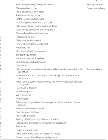
Table 4 Industry classification

Sector number Description Industry group

1 Agriculture, hunting, forestry, and fishing Primary industry

2 Mining and quarrying Secondary industry

3 Food, beverages, and tobacco 4 Textiles and textile products 5 Leather, leather, and footwear 6 Wood and products of wood and cork 7 Pulp, paper, paper, printing, and publishing 8 Coke, refined petroleum, and nuclear fuel 9 Chemicals and chemical products 10 Rubber and plastics

11 Other nonmetallic mineral 12 Basic metals and fabricated metal 13 Machinery, nec

14 Electrical and optical equipment 15 Transport equipment

16 Manufacturing, nec; recycling 17 Electricity, gas, and water supply 18 Construction

19 Sale, maintenance, and repair of motor vehicles and motorcycles; retail

sale of fuel Tertiary industry

20 Wholesale trade and commission trade, except of motor vehicles and motorcycles

21 Retail trade, except of motor vehicles and motorcycles; repair of house-hold goods

22 Hotels and restaurants 23 Inland transport 24 Water transport 25 Air transport

26 Other supporting and auxiliary transport activities; activities of travel agencies

27 Post and telecommunications 28 Financial intermediation 29 Real estate activities

30 Renting of M&Eq and other business activities 31 Public admin and defense; compulsory social security

32 Education

33 Health and social work

Table 5 Income classification of countries examined in the study

Country number Country Abbreviation Income group

1 Australia AUS High-income group

2 Austria AUT

3 Belgium BEL

4 Canada CAN

5 Cyprus CYP

6 Czech Republic CZE

7 Germany DEU

8 Denmark DNK

9 Spain ESP

10 Estonia EST

11 Finland FIN

12 France FRA

13 UK GBR

14 Greece GRC

15 Ireland IRL

16 Italy ITA

17 Japan JPA

18 Korea KOR

19 Lithuania LTU

20 Luxembourg LUX

21 Latvia LVA

22 Malta MLT

23 Netherlands NLD

24 Poland POL

25 Portugal PRT

26 Russia RUS

27 Slovakia SVK

28 Slovenia SVN

29 Sweden SWE

40 Taiwan TWN

30 USA USA

31 Bulgaria BGR Middle-income group

32 Brazil BRA

33 China CHN

34 Hungary HUN

35 Mexico MEX

36 Romania ROM

37 Turkey TUR

38 Indonesia IDN Low-income group

39 India IND

Received: 21 January 2016 Accepted: 19 July 2016

References

Ang BW (2004) Decomposition analysis for policymaking in energy: which is the preferred method? Energy Policy 32:1131–1139

Ang BW, Liu FL, Chew EP (2003) Perfect decomposition techniques in energy and environmental analysis. Energy Policy 31:1561–1566

Casler SD, Rose A (1998) Carbon dioxide emissions in the U.S. economy: a structural decomposition analysis. Environ Resour Econ 11:349–363

Davis SJ, Peters GP, Caldeira K (2011) The supply chain of CO2 emissions. Proc Natl Acad Sci USA 108:18554–18559 Dietzenbacher E, Los B (1997) Analyzing decomposition analysis. In: Simonovits A, Steenge AE (eds) Prices, growth and

cycles. Macmillan, London, pp 108–131

Dietzenbacher E, Los B (1998) Structural decomposition technique: sense and sensitivity. Econ Syst Res 12:307–323 Dietzenbacher E, Hoen AR, Los B (2000) Labor productivity in Western Europe 1975–1985: an intercountry analysis. J Reg

Sci 40:425–452

Dietzenbacher E, Los B, Stehrer R, Timmer M, de Vries G (2013) The construction of World Input–Output Tables in the WIOD project. Econ Syst Res 25:71–98

Hertwich EG, Peters GP (2009) Carbon footprint of nations: a global, trade-linked analysis. Environ Sci Technol 43:6414–6420

Hoekstra R, van den Bergh JJCJM (2003) Comparing structural and index decomposition analysis. Energy Econ 25:39–64 IPCC (2014) Climate change 2014: mitigation of climate change. https://www.ipcc.ch/report/ar5/wg3/

Kagawa S, Inamura H (2001) A structural decomposition of energy consumption based on a hybrid rectangular input– output framework: Japan’s case. Econ Syst Res 13:339–363

Kagawa S, Yuriko G, Sangwon S, Keisuke N, Yuki K (2012) Accounting for changes in automobile gasoline consumption in Japan: 2000–2007. J Econ Struct 1(9):1–27

Leontief W, Ford D (1972) Air pollution and economic structure: empirical results of input-output computations. In: Brody A, Carter A (eds) Contributions to input–output analysis. North-Holland, Amsterdam, pp 9–30

Levinson A (2009) Technology, international trade, and pollution from US manufacturing. Am Econ Rev 99:2177–2192 Lin X, Polenske KR (1995) Input–output anatomy of China’s energy use changes in the 1980s. Econ Syst Res 7:67–84 Nansai K, Kagawa S, Suh S, Inaba R, Moriguchi Y (2007) Simple indicator to identify the environmental soundness of

growth of consumption and technology: “Eco-velocity of consumption”. Environ Sci Technol 41:1465–1472 Nansai K, Kagawa S, Suh S, Fujii M, Inaba R, Hashimoto S (2009) Material and energy dependence of services and its

implications for climate change. Environ Sci Technol 43:4241–4246

Okamoto S (2013) Impacts of growth of a service economy on CO2 emissions: Japan’s case. J Econ Struct 2:1–21 Oshita Y (2012) Identifying critical supply chain paths that drive changes in CO2 emissions. Energy Econ 34:1041–1050 Park SH (1992) Decomposition of industrial energy consumption: an alternative method. Energy Econ 13:265–270 Peters G, Minx J, Weber CL, Edenhofer O (2011) Growth in emission transfers via international trade from 1990 to 2008.

Proc Natl Acad Sci 108:8903–8908

Proops JLR (1984) Modelling the energy-output ratio. Energy Econ 6:47–51

Rose A, Casler SD (1996) Input–output structural decomposition analysis: a critical appraisal. Econ Syst Res 8:33–62 Rose A, Chen CY (1991) Sources of change in energy use in the U.S. economy, 1972–1982: a structural decomposition

analysis. Resour Energy 13:1–21

Sun JW (1998) Changes in energy consumption and energy intensity: a complete decomposition model. Energy Econ 20:85–100

Tian X, Changb M, Shia F, Tanikawaa H (2014) How does industrial structure change impact carbon dioxide emissions? A comparative analysis focusing on nine provincial regions in China. Environ Sci Policy 37:243–254

Timmer MP, Dietzenbacher E, Los B, Stehrer R, de Vries GJ (2015) An illustrated user guide to the world input–output database: the case of global automotive production. Rev Int Econ 23:575–605

United Nations (1999) Handbook of input–output table compilation and analysis, studies in method series F, vol 74. U. N, New York

Voigt S, De Cian E, Schymura M, Verdolini E (2013) Energy intensity developments in 40 major economies: structural change or technology improvement? Energy Econ 41:47–62

Wier M (1998) Sources of changes in emissions from energy: a structural decomposition analysis. Econ Syst Res 10:99–112

Wood R, Lenzen M (2009) Structural path decomposition. Energy Econ 31:335–341

World Bank (2013). http://siteresources.worldbank.org/DATASTATISTICS/Resources/CLASS.XLS. Accessed 26 July 2016 Xu Y, Dietzenbacher E (2014) A structural decomposition analysis of the emissions embodied in trade. Ecol Econ