Estimating local commuting patterns from geolocated Twitter data

(1)

R E G U L A R A R T I C L E

Open Access

Estimating local commuting patterns from

geolocated Twitter data

Graham McNeill, Jonathan Bright

*

_{and Scott A Hale}

*_{Correspondence:}

[email protected] Oxford Internet Institute, University of Oxford, Oxford, United Kingdom

Abstract

The emergence of large stores of transactional data generated by increasing use of digital devices presents a huge opportunity for policymakers to improve their knowledge of the local environment and thus make more informed and better decisions. A research frontier is hence emerging which involves exploring the type of measures that can be drawn from data stores such as mobile phone logs, Internet searches and contributions to social media platforms and the extent to which these measures are accurate reflections of the wider population. This paper contributes to this research frontier, by exploring the extent to which local commuting patterns can be estimated from data drawn from Twitter. It makes three contributions in particular. First, it shows that heuristics applied to geolocated Twitter data offer a good proxy for local commuting patterns; one which outperforms the current best method for estimating these patterns (the radiation model). This finding is of particular significance because we make use of relatively coarse geolocation data (at the city level) and use simple heuristics based on frequency counts. Second, it investigates sources of error in the proxy measure, showing that the model performs better on short trips with higher volumes of commuters; it also looks at demographic biases but finds that, surprisingly, measurements are not significantly affected by the fact that the demographic makeup of Twitter users differs significantly from the population as a whole. Finally, it looks at potential ways of going beyond simple frequency heuristics by incorporating temporal information into models.

Keywords: transport; mobility; social media; geolocation

1 Introduction

Population movement is a key issue for contemporary policymakers, who need to optimise transport infrastructures and services which are under ever increasing pressure. However these policymakers often operate in an information scarce environment: existing mea-surement instruments such as transport surveys (which may involve stopping people as they cross the border or drive through a speciﬁc road) are time consuming and expensive as well as being a source of frustration for the local population. Hence data collection is infrequent and decisions are often based on incomplete, out-of-date estimates.

The emergence of social media as a potential window on population movement oﬀers a huge opportunity in this regard [–]. Data from social media platforms is often available to policymakers at relatively low cost, sometimes even for free. It can also be sourced without creating disruption, as the data is generated as a byproduct of interaction with

(2)

the social media platform. Furthermore, it is available in huge quantities on an ongoing basis, meaning that real time changes can be tracked. Hence the potential of social media as a secondary data source is considerable.

The availability of social media data has made it a rich area for academic research on the extent to which it can oﬀer census like indicators in a whole variety of areas such as un-employment [], consumer behaviour [], stock market movements [], health outcomes [, ] and elections [, ]. Some initial work has started to emerge in the area of popula-tion movement in particular. For example Liuet al.[] have investigated the correlation between population and Twitter data in Australia, ﬁnding that at large scales population levels could be estimated from the prevelance of geolocated Twitter content. Hawelkaet al.

[] meanwhile, looked at international population mobility, tracing the number of inter-national tourists, again based on geolocated Twitter data; whilst Beiróet al.took a similar approach to domestic commuting patterns []. Finally, a variety of studies have success-fully modelled intra-city movement patterns using Twitter and Foursquare check-in data [–]. However, while these initial results are promising, much more remains to be done in terms of understanding the extent to which social media can be used systematically as an accurate indicator of population movement.

The aim of this article is to build on this existing literature by examining the extent to which local commuting patterns in the United Kingdom can be inferred from data sourced from Twitter. We make three contributions in particular. First, we show that heuristics applied to geolocated Twitter data offer a good proxy for local commuting patterns; one which outperforms the major existing method for estimating these patterns (the radia-tion model). This finding is of particular significance because we make use of relatively coarse geolocation data (at the city level) and use simple heuristics based on frequency counts. Second, we investigate sources of error in our proxy measure, showing that the model performs better on short trips with higher volumes of commuters; we also look at demographic biases, and find that, surprisingly, our measurements are not significantly af-fected by the fact that the demographic makeup of Twitter users differs significantly from the population as a whole. Finally, we look at potential ways of going beyond our simple heuristics by incorporating temporal information into our models.

The rest of the article is structured in the following way. Section  sets out the meth-ods and data, explaining the means of estimating commuting ﬂow from Twitter and how these estimates are validated against a ground truth census dataset. It also outlines the radiation model of commuting which we make use of as a benchmark. Section  presents the results of the model, comparing our Twitter estimates to the benchmark and also ex-ploring sources of bias and error in the estimation. Section , ﬁnally, explores temporal based extensions to the model.

2 Methods and data

(3)

people send tweets from their mobile phone []). Although historic studies of geotagged tweets have made use of exact co-ordinate data, currently the majority of geotagged data produced by the social media network is relatively coarse, accurate only to the city or municipality level.a

Geolocated tweets indicate, of course, where a user currently is, rather than anything about any journey they may make. However, it seems reasonable to assume that, whilst making use of the social network, many people may tweet from both their home and work locations. Hence a pattern of geotagged tweets, over a period of time, ought to contain information about patterns of commuting. Of course, there will be a certain amount of noise in the data as people will tweet from other locations: on their way to/from work, from restaurants, on holiday, etc. Furthermore, not all Twitter users will have a job, nor will all jobs require regular commuting. One of the central questions in this article is to observe the extent to which commuting patterns can be inferred in spite of this noise.

Going from geolocated tweets to commuting patterns requires us to choose a heuristic for deciding which location is a ‘home’ location and which location is a ‘work’ location for each user, based on a pattern of geolocated tweets which may come from a variety of areas. There is a growing literature on the best way of inferring these locations from a pattern of digital trace data such as tweets or mobile phone calls [–]. We make use of arguably the simplest of these: a frequency count (although in Section  we experiment with ways of improving on this simple method by making use of temporal information, it is helpful to ﬁrst observe the amount of signal that can be extracted from the simplest possible heuristics applied to the data). Hence, the area that a user most frequently tweets from is assumed to be their home location; the second most frequent is assumed to be their work location (users which have a tie for home and work location are discarded). All other locations are assumed to be areas visited which are unrelated to either living or working. To account for users who live and work in the same area, we use a thresholdλ: if more thanλ%of tweets are sent from the same area, we assume the user both lives and works in that area. In our results section, we experiment with diﬀerent values ofλto test the sensitivity of the model to this threshold.

Having assigned users to home and work locations, we can construct a commuter ﬂow matrix T:

Tij=twij, ()

wheretwijis the number of users which have their home in locationiand work in loca-tionj.

We take as our ground truth dataset commuting data from the  UK census.bThe census gives data on commuting volumes within and between ‘local authorities’, which are administrative regions within the UK (of which there are  in totalc_{). By comparing} es-timates from our Twitter model to actual numbers derived from the census, we can assess the accuracy of commuting predictions derived from Twitter. The census also provides information on commuting volumes across diﬀerent demographic groups, which allow us to assess demographic variation in the accuracy of our results.

(4)

used gravity model (e.g.[, , ]), and the more recent radiation model []. In this paper, we opt to use the radiation model as a benchmark, as it has been shown to outper-form the gravity model. It is also well-suited to our purposes since it is parameter-free and only requires basic information about each area. Hence it oﬀers a reasonable comparison to our context, where the aim is to infer commuting patterns with only a minimal amount of observational data.

The standard radiation model estimates the commuter ﬂow matrix T using:

Tij=ciProb(work =j|home =i) =ci

ninj (ni+sij)(ni+nj+sij)

,

where:

• T_ijis theijth entry ofT, the number of commuters who live in areaiand work in area

j;

• ciis the total number of outward commuters who live in areai; • niis the population in areaiandnjis the population in areaj;

• sijis the population within a circle centered at areaiand with a radius equal to the distance between areasiandj(the populations of areasiandjare not included). The model assumes that the number of outward or external commuters from an area is proportional to its population. Hence,ci=C(ni/N) whereCis the total number of outward commuters in the population andNis the total population (given byN=_ini). IfCis unknown, the model can estimateProb(work =j|home =i), but not absolute commuter numbers. It is worth noting that the radiation model does not oﬀer a prediction for internal commuting,i.e.the number of people who live and work in the same area, a point to which we will return below.

Yanget al.[] have introduced a -parameter variant of the radiation model, which has been shown to outperform the parameter-free version. We hence also include this model in our analysis. The estimated ﬂow for the -parameter model is given by:

T_ij=ci

[(aij+nj)α–aαij](nαi + ) (aα

ij+ )[(aij+nj)α+ ]

, ()

whereaij=ni+sij. Yanget al.construct the parameterαso that it varies with the average size of regions for which commuting is being estimated. In particular, they calculateα

using:

α=

l

 [km] .

, ()

wherelis the mean ‘length’ of regions under consideration, deﬁned as the square root of their area (for our particular case of UK local authorities,lis equal to  km).

(5)

tweets from within a bounding box around the British Isles.dIt is worth remarking that the choice of a full year period is signiﬁcant. We expect (and indeed we found) that user engagement with the platform is bursty [], meaning that a large time window is required to build up a consistent pattern of tweets for one user. However, using a year long period means that we are capturing certain types of bias in our data: for example, we may pick up occasional long distance movements, such as students moving between their homes and places of study (as found by []), which shorter time spans might avoid.

We logged rate limiting messages from the Twitter Streaming API and found that few tweets were omitted per day due to rate limiting. We experienced no rate limiting at all for  days and only slight rate limiting on other days (median . tweets lost on days with rate limiting messages). Power interruptions and network connectivity resulted in addi-tional data loss, but there is no indication of any systematic bias from these interruptions. During our time window, ,, individual users sent a geolocated tweet which fell within our bounding box.

The distribution of user activity is, as might be expected, heavy tailed, with a majority of users relatively inactive. We expect that users who tweet more frequently will give a more accurate signal about their home and work locations, hence we decided to impose a number of filters on the dataset to only include users of the platform who had a relatively high level of engagement. We make use of three filters in particular. First, we discarded users who had less than  tweets, as a kind of minimum threshold for extracting any kind of signal from the pattern of user engagement. Second, we discarded users who did not have either two tweets in two separate local authorities, or greater than theλthreshold of tweets within one local authority (meaning it could be assigned as both a home and work location): again, this was done to set a minimum threshold for extracting signal from a pattern of user engagement. Finally, we discarded users whose first and last tweets in their detected locations were less than  days apart (to try and eliminate, for example, people who only sent a short burst of tweets from a holiday destination). Application of these filters resulted in a large number of low-intensity users being discarded. After these steps the exact size of the dataset varied with theλthreshold, from just over , forλ= . to just over , forλ= .. We discuss the potential impact of this filtering more in our results section below.

In order to assign living and working locations to users, we ﬁrst assigned each geolocated tweet to a local authority area. This assignment was achieved in one of two ways. When exact coordinates were included with the tweet, assignment was simple, as any pair of co-ordinates will fall within only one local authority. If co-co-ordinates are not included, what Twitter includes instead is a bounding box around a given place or region of geographic interest (for example, a city, a county or even a country); Twitter also includes information about the type of bounding box.e_{If the type of place is deﬁned as a ‘city’ we use the centroid} of the bounding-box as our point for geolocation, on the assumption that the majority of cities do not cross local authority boundaries (it is worth noting that a ‘city’ in this context also refers to an area of London). In total, we were able to assign % of tweets to a local authority, or  million tweets in total. Geolocated tweets which could not be assigned are those where the area of geolocation was too high to meaningfully assign to a local authority (for example, tweets can be geolocated to ‘United Kingdom’ or ‘East England’).

(6)

the ‘correct’ name. Furthermore, some bounding boxes may cross local authority bound-aries, making the centroid an unreliable means of distinguishing location. Nevertheless, we expect the process to be broadly accurate. This is something supported by an observed strong correlation (r= .) between geolocated tweets and the population of each local authority (a finding which also offers further confirmation for the results from []).

3 Modelling commuting with Twitter

We will now move on to discuss the results of the study. We will begin by looking at how predictions from our Twitter model compare to the ground truth census data; and also whether the accuracy of Twitter based predictions can improve on predictions from the radiation model. Following [] and [], we use the ‘common part of commuters’ [CPC] score based on the Sørensen index [] to assess the accuracy of commuting ﬂow esti-mates. A CPC score essentially compares the similarity of two matrices, L andL, and is given by the following equation:

CPC(L,L) = K

i,j=min(Lij,Lij) K

i,j=[L +L]ij

, ()

whereKis the number of rows in the matrix (in our case the number of local authority areas). CPC scores lie in [, ] with  indicating perfect agreement,i.e.L=L. We also calcu-lated all our results using Cosine distance and the Pearson product-moment correlation, to check whether our ﬁndings were sensitive to the metric used. The conclusions from these other two measures were essentially identical, and hence have not been reported here.

As described above, estimates from the radiation model are typically normalised, with rowitranformed to sum toci=C(ni/N), whereCis the overall volume of commuting,niis the population of the local authority represented by rowi, andNis the overall population. Here, we perform this normalisation on both the estimates from the radiation model and the Twitter model, to make results generated comparable.Cis calculated by summing the commuting matrix from the census; we also make use of local authority population ﬁgures from the census to calculateniandN.

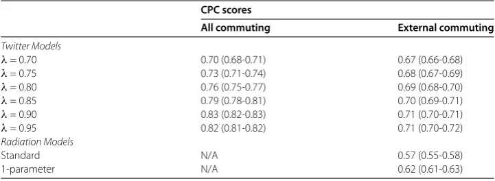
Table  shows the CPC values for the Twitter-based estimates, with values ofλvarying between . and ., and both variants of the radiation model (using equation () to estimate the parameter). As mentioned above, the radiation model does not oﬀer an es-timate for internal commuting (i.e.the number of people who live and work in the same area), whereas the Twitter model does. To properly compare the two approaches, we hence also produced a version of the Twitter model which considers only external commuting:

i.e.the diagonal entries of the ﬂow matrix are set to zero. All estimates have bootstrapped % conﬁdence intervals generated from , bootstrap samples.

(7)

Table 1 CPC scores for comparisons of the Twitter model and the radiation models to commuting data from the census. Brackets contain bootstrapped 95% conﬁdence intervals

CPC scores

All commuting External commuting

Twitter Models

λ= 0.70 0.70 (0.68-0.71) 0.67 (0.66-0.68)

λ= 0.75 0.73 (0.71-0.74) 0.68 (0.67-0.69)

λ= 0.80 0.76 (0.75-0.77) 0.69 (0.68-0.70)

λ= 0.85 0.79 (0.78-0.81) 0.70 (0.69-0.71)

λ= 0.90 0.83 (0.82-0.83) 0.71 (0.70-0.71)

λ= 0.95 0.82 (0.81-0.82) 0.71 (0.70-0.72)

Radiation Models

Standard N/A 0.57 (0.55-0.58)

1-parameter N/A 0.62 (0.61-0.63)

improves on existing freely available models. This is especially signiﬁcant if we consider both the simplicity of the location assignment technique, and the relatively coarse grained nature of the data (based on relatively wide area bounding boxes). Finally, higher values of

λare associated with higher CPC scores. This might indicate that, typically, users make much more use of the social media network when they are at home rather than at work: hence even a small amount of tweets in another area might indicate a pattern of external commuting. However, it is worth noting that this may also be related to the fact that, as described above, more users are discarded at higher levels ofλ.

In addition to this general measurement of the accuracy of the Twitter model, it is also worth exploring some of the sources of error in the predictions it generates. These errors are interesting from a scientiﬁc point of view, but they are also of policy relevance. For instance, if Twitter data oﬀers better estimates for certain demographic groups, certain areas, or certain types of trip, then the people or places for whom the estimates are better may be favoured if Twitter data is used in policy decisions (for example, transport infras-tructures might be unknowingly adapted more toward the needs of those who make more use of Twitter).

We explore sources of error in the model in a variety of ways below: in each case we make use of the best performing model identified, which was the Twitter model with internal commuting included and withλ= .. The first source of error we investigated was the volume of commuting between local authority pairs: we might expect local-authority pairs that share lots of commuters to be estimated better than pairs that have just a few com-muters, as the signal will be stronger and hence less affected by noise in the data. Figure  investigates this possibility, by showing a heatmap of the estimates for the Twitter-based approach against the census data (estimates for the one parameter radiation model are also included for the purposes of comparison).

(8)

Figure 1 Estimated commuter ﬂow. (a)1-parameter radiation model.(b)Twitter model (λ= 0.90). Axes are log transformed, with all data points incremented by 1 before transformation.

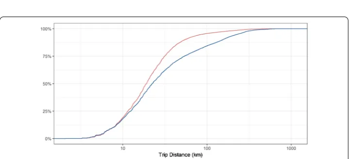
Figure 2 Empirical cumulative distribution of commuting trip distances.Red: census data. Blue: Twitter model.

volume of commuters it is much less signiﬁcant: less than % of total commuters travel on these low intensity routes.

(9)

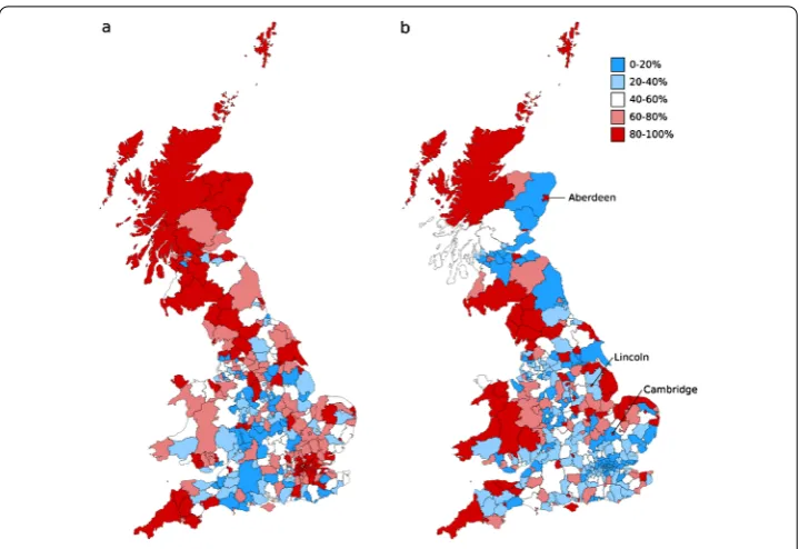
es-Figure 3 Absolute error in the estimated outward commuting distributions. (a)1-parameter radiation model.(b)Twitter model (λ= 0.90). Color: quintiles for the combined set of errors from both approaches.

timate. This speculation is supported by [], which has shown that Twitter data can also be used to estimate long term internal migration patterns (the study focussed particularly on students leaving their home town to go to university). There is, in other words, clearly a trade oﬀ in terms of using social media data: using a longer time period allows more data to be built up, and hence potentially a stronger signal; but it also introduces new types of bias which otherwise would not be present.

We will next look at the geographic distribution of error within the models. We might expect a variety of types of geographic variation in error: for example we might observe better predictions to be available for densely populated city areas for which there is more data. In order to investigate this, we rewrite equation () as:

CPC(L,L) =  – K

i,j=|Lij–Lij| K

i,j=[L +L]ij

. ()

The numerator in equation () is a sum over prediction errors; so, we can look at the error associated with a given local authority by fixingiand summing overjto get the out-ward commuting error. Since the total number of outout-ward commuters is different for each local authority, we first normalize each row of L andLto sum to  and hence, consider the outward flow probability distribution for each local authority. The results are visualized in Figure , which contains results both from the Twitter model and the -parameter ra-diation model for comparison.

(10)

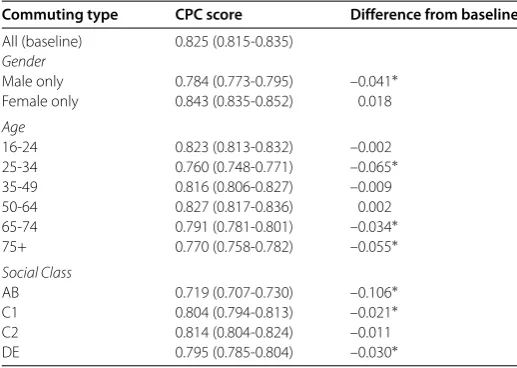
Table 2 CPC scores for the estimated Twitter commuting matrix (λ= 0.90) compared against census commuting volumes divided by gender, age and social class. Internal commuting is included. Brackets contain bootstrapped 95% conﬁdence intervals. * indicates the conﬁdence interval for the category being considered does not overlap with the interval for the full census

Commuting type CPC score Difference from baseline

All (baseline) 0.825 (0.815-0.835)

Gender

Male only 0.784 (0.773-0.795) –0.041∗ Female only 0.843 (0.835-0.852) 0.018

Age

16-24 0.823 (0.813-0.832) –0.002 25-34 0.760 (0.748-0.771) –0.065∗ 35-49 0.816 (0.806-0.827) –0.009

50-64 0.827 (0.817-0.836) 0.002

65-74 0.791 (0.781-0.801) –0.034∗ 75+ 0.770 (0.758-0.782) –0.055∗

Social Class

AB 0.719 (0.707-0.730) –0.106∗

C1 0.804 (0.794-0.813) –0.021∗

C2 0.814 (0.804-0.824) –0.011

DE 0.795 (0.785-0.804) –0.030∗

poor estimates of the small amounts of commuting that go out from these cities into the surrounding countryside (by contrast, the amounts of commuting into these cities is well estimated, something shown by the fact that the areas surrounding the cities are typically blue). It is worth noting that within the large metropolitan area of London, the Twitter model performs well in absolute terms, and also much better than the radiation model, which does quite poorly in this area (something also found by []).

A ﬁnal area of potential error we considered concerned the impact of demographic fac-tors. Twitter users are not demographically representative of the general population [, ], and furthermore Twitter users who geotag their tweets are not even representative of Twitter users more generally [, ]. We might expect this bias in the type of user included in the model to distort the results; for example, Twitter commuting estimates might be better for groups which are well represented on Twitter. In order to consider the impact of demographics on commuting predictions, we make use of further census data which describes the level of commuting between local authority pairs for a variety of dif-ferent socio-demographic categories. In particular, commuting is divided up by gender, by age group, and by social class. For each of these demographic variables, we compare the performance of our predictor with the baseline performance for all types of commuting generated in Section  (again withλ= .).

(11)

less, and in no categories was the observed CPC score lower than .. From this we con-clude that, even though the users of Twitter might be demographically biased, this does not hamper to a large extent our ability to infer mostly accurate commuting patterns from the data.

4 Extending the Twitter model

As we have highlighted, the simple model using Twitter data oﬀers a good proxy for local commuting patterns, but not a perfect one. In this further analytical section, therefore, we want to consider ways of extending the model. Our current model is simplistic: it makes use of a mere frequency count of the geographic locations of tweets to assign individuals to a home and work location. However, Twitter data contains much more information than just geographic locations, and including this extra information might improve our predictions. In this section, we explore one particular avenue, looking at whether temporal information might oﬀer an improvement in accuracy. Temporal information is of course something which is already made use of in a variety of existing works on trace data [–, ].

Working (and hence commuting) typically follows temporal patterns. Hence it might be possible to improve the accuracy of our assignment of home and work locations by considering whether a user’s tweets are being sent during the typical working day. To test this possibility, we of course ﬁrst need to deﬁne the limits of the working day. In Figure , we explore the extent to which we can do this on the basis of our Twitter data, by looking at how patterns of tweets within our data vary over time.

We begin by looking at whether there is any variation between weekdays, where the ma-jority of work occurs, and the weekend. Figure (a) and (b) show the temporal distribution of tweets on Saturday-Sunday compared to Monday-Friday for each local authority. Fig-ure (c) shows the means of the weekend and weekday distributions. As we might expect there appear to be slightly different patterns of Twitter usage on weekends and weekdays, with weekday use characterised by a sharper evening peak (the period which runs ap-proximately from :-:) and flatter use levels during the daytime (apap-proximately :-:). This suggests that patterns of geolocated Twitter usage are different dur-ing the workdur-ing week, hence only usdur-ing data created durdur-ing weekdays might improve the accuracy of the Twitter model.

We will now move on to exploring temporal ﬂuctuations during the day. In Figure (d), we cluster the distributions in Figure (b) usingK-medoids clustering (K= ) with the earth-mover’s distance [], a well-used metric that computes the cost of transforming one distribution into another. It is notable that one cluster (shown in blue) is character-ized by fewer tweets during the daytime and a higher peak in the evenings, whilst the other (shown in red) has comparatively more tweets during the day and less in the evening. This could suggest that the blue cluster represents local authorities with high outward commut-ing and the red cluster represents authorities with high inward commutcommut-ing. As a means of validating this proposition, we compute the ratio of inward to outward commuters for each authority and ﬁnd the geometric mean of these ratios for each cluster (we use the ge-ometric mean here as it is more appropriate for ratio data). The means are . and .: on average, inward commuting is % of outward commuting in the red cluster, but only % in the blue cluster, which seems to support our assumption.

(12)

Figure 4 Temporal distribution of tweets for each local authority. (a)Saturday and Sunday. (b)Monday-Friday.(c)Mean of weekend and weekday distributions.(d)Clustering local authorities on Monday-Friday distributions usingK-medioids (K= 2) with the earth-mover’s distance.(e)Cluster membership of local authorities.

about the appropriate time window to use for the typical working day. In Figure (d), the two clusters intersect at around : and :, suggesting this time period could be used as delimiting the typical working day. The clusters are also particularly clearly separated during the periods :-: and :-:, which suggests that focusing on these times as a kind of ‘restricted’ working day may be optimal in terms of identifying work and home locations respectively. We experiment with the use of both of these approaches to deﬁning the working day below.

(13)

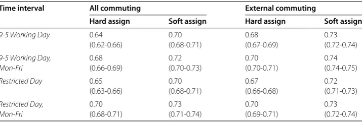
Table 3 CPC for Twitter-based estimates using different time-based heuristics, for both hard and soft assignment techniques. Brackets contain bootstrapped 95% conﬁdence intervals. The restricted day only considers tweets from 10:00-15:00 when calculating the work location, and tweets from 20:00-23:00 when calculating the home location

Time interval All commuting External commuting

Hard assign Soft assign Hard assign Soft assign

9-5 Working Day 0.64 0.70 0.68 0.73

(0.62-0.66) (0.68-0.71) (0.67-0.69) (0.72-0.74)

9-5 Working Day, 0.68 0.72 0.70 0.74

Mon-Fri (0.66-0.69) (0.70-0.73) (0.70-0.71) (0.74-0.75)

Restricted Day 0.65 0.70 0.67 0.72

(0.63-0.66) (0.68-0.71) (0.66-0.68) (0.71-0.73)

Restricted Day, 0.70 0.73 0.70 0.73

Mon-Fri (0.68-0.71) (0.71-0.74) (0.69-0.71) (0.72-0.74)

with similar amounts of tweets ought to have less certainty in them than users who had one work area which had a very clear majority.

In order to incorporate the uncertainty in assigning a home and work location to each user we consider a method of soft assignment by creating a ‘location matrix’ Lufor each user, which is given by:

L_u= huwTu,

where huand wuare the normalized distributions of home and work tweet counts for user

urespectively. Hence, we can interpret the entries of Luas: [Lu]ij= [hu]i[wu]j

=Prob(live =i)Prob(work =j) =Prob(live =i, work =j).

To estimateProb(live =i, work =j) for the population, we take the mean over allUusers:

L= 

U

u=

Lu.

The rows of L are then normalized as before.f

Table  shows the CPC scores based on the temporal heuristics discussed above. Results are provided both for the Twitter model based on all commuting and the model which is based only on external commuting. For each of these two types of model, we show results using the hard assignment method which we used in Section  (whereby the top two lo-cations from which a user tweets are used as their home and work lolo-cations respectively) and the soft assignment method described above which incorporates uncertainty.

(14)

Furthermore, the best performing heuristics in Table  only oﬀer a modest improvement on the estimations of external commuting developed with simpler heuristics (Table ), and no improvement when internal commuting is considered. This is perhaps surprising: it may suggest that temporal information is not as valuable as we might have expected when estimating diﬀerent location patterns. However, it may also be related to the fact that, as people appear to moderate their Twitter usage during working hours, the signal contained in temporal information is already largely captured by our simple frequency counts.

5 Conclusion

In this paper we have set out to examine the extent to which Twitter data can be used to estimate local commuting flows, thus building on the nascent literature that seeks to extract reliable population indicators from social media data. We have shown that simple heuristics applied to Twitter data offer good approximations of local commuting patterns; approximations that outperform the current benchmark for commuter flow estimation models (the radiation model). We explored the sources of error in these estimations, and found that Twitter was more reliable at estimating large commuting flows over short dis-tances, and less reliable at estimating small amounts of long range commuting. We found some evidence of geographic and demographic biases in the data, though these biases were not severe. We also explored potential extensions to the models, but in the end found that simple frequency heuristics largely outperformed more complicated models using tem-poral information. In conclusion, we would argue that this paper highlights again the po-tential of freely created and distributed social media data for understanding more about local populations.

Funding

This project was supported by funding from InnovateUK under grant number 52277-393176 and the NERC under grant number NE/N00728X/1.

Abbreviations

OD: Origin-Destination. API: Application Programming Interface. CPC: Common Part of Commuters.

Availability of data and materials

Data supporting the publication will be made available in Oxford’s institutional repository following publication.

Ethics approval and consent to participate

We conﬁrm that this study has received ethical approval from the University of Oxford’s Ethics Review board (case ref: SSH OII C1A 16 076).

Competing interests

We declare no competing interests.

Consent for publication Not applicable.

Authors’ contributions

SH collected the data for the manuscript, whilst GM and JB produced the analysis. All authors contributed equally to the drafting of the manuscript. All authors read and approved the ﬁnal manuscript.

Endnotes

a _{For more details on current geotagging practices in the Twitter Streaming API see:}

https://twittercommunity.com/t/foursquare-location-data-in-the-api/36065

b _{https://wicid.ukdataservice.ac.uk/}

c _{In the census commuting data (and throughout this article), Westminster and the City of London are treated as a}

single local authority, as are Cornwall and the Isles of Scilly.

d _{The coordinates used form a rectangle with a lower-left corner at –13.4139, 49.1621, and a top-right corner at}

(15)

e _{It is worth noting that the time period considered starts after Twitter began promoting the inclusion of ‘place’ in}

tweets rather than the exact latitude-longitude coordinates. These places are represented as bounding boxes in the data. From earlier data, we observed an 80% decrease in exact-geotagged tweets in April 2015, though the the overall number of geotagged tweets (i.e.exact or place) remained stable.

f _{Extending the ﬁltering from Section 3, entries of}_hu_and_wu_{that are not associated with tweets spanning longer}

than a 30 day period are reset to 0 before the vectors are normalized. Users that do not have at least one non-zero entry in bothhuandwuare discarded. Depending on the precise time-windows used, 75-85% of users are discarded, leaving 287,000-496,000 users.

Publisher’s Note

Springer Nature remains neutral with regard to jurisdictional claims in published maps and institutional aﬃliations.

Received: 21 February 2017 Accepted: 14 September 2017 References

1. Mayer-Schönberger V, Cukier K (2013) Big data: a revolution that will transform how we live, work, and think. John Murray, London

2. Lazer D, Pentland A, Adamic L, Aral S, Barabasi AL, Brewer D, Christakis N, Contractor N, Fowler J, Gutmann M, Jebara T, King G, Macy M, Roy D, Van Alstyne M (2009) Life in the network: the coming age of computational social science. Science 323(5915):721-723

3. Voigt C, Bright J (2016) The lightweight smart city and biases in repurposed big data In: The second international conference on human and social analytics (HUSO 16)

4. Llorente A, Garcia-Herranz M, Cebrian M, Moro E (2014) Social media ﬁngerprints of unemployment. PLoS ONE 10(5):e0128692

5. Goel S, Hofman JM, Lahaie S, Pennock DM, Watts DJ (2010) Predicting consumer behavior with web search. Proc Natl Acad Sci USA 107(41):17486-17490

6. Curme C, Preis T, Stanley HE, Moat HS (2014) Quantifying the semantics of search behavior before stock market moves. Proc Natl Acad Sci USA 111(32):11600-11605

7. Broniatowski DA, Paul MJ, Dredze M (2013) National and local inﬂuenza surveillance through Twitter: an analysis of the 2012-2013 inﬂuenza epidemic. PLoS ONE 8(12):e83672

8. Kostkova P, Szomszor M, St Louis L (2009) #swineﬂu: the use of Twitter as an early warning and risk communication tool in the 2009 swine ﬂu pandemic. ACM Trans Manag Inform Syst (TMIS) 5(2):8

9. Yasseri T, Bright J (2016) Wikipedia traﬃc data and electoral prediction: towards theoretically informed models. EPJ Data Sci 5:22

10. Yasseri T, Bright J (2014) Can electoral popularity be predicted using socially generated big data?. IT, Inf Technol 10.1515/itit-2014-1046

11. Liu J, Zhao K, Khan S, Cameron M, Jurdak R (2014) Multi-scale population and mobility estimation with geo-tagged tweets. In: 31st IEEE international conference on data engineering workshops, pp 83-86

12. Hawelka B, Sitko I, Beinat E, Sobolevsky S, Kazakopoulos P, Ratti C (2014) Geo-located Twitter as proxy for global mobility patterns. Cartogr Geogr Inf Sci 41(3):260-271

13. Beiró MG, Panisson A, Tizzoni M, Cattuto C (2016) Predicting human mobility through the assimilation of social media traces into mobility models. EPJ Data Sci 5(1):17

14. Noulas A, Scellato S, Lambiotte R, Pontil M, Mascolo C (2012) A tale of many cities: universal patterns in human urban mobility. PLoS ONE 7(5):e37027

15. Liu Y, Sui Z, Kang C, Gao Y (2014) Uncovering patterns of inter-urban trip and spatial interaction from social media check-in data. PLoS ONE 9(1):e86026

16. Mcardle G, Furey E, Lawlor A, Pozdnoukhov A (2014) Using digital footprints for a city-scale traﬃc simulation. ACM Trans Intell Syst Technol (TIST) 5(3):41

17. Morstatter F, Pfeﬀer J, Liu H, Carley KM (2013) Is the sample good enough? Comparing data from Twitter’s streaming API with Twitter’s ﬁrehose. In: Proceedings of the seventh international AAAI conference on weblogs and social media

18. Graham M, Hale SA, Gaﬀney D (2014) Where in the world are you? Geolocation and language identiﬁcation in Twitter. Prof Geogr 66(4):568-578

19. Alexander L, Jiang S, Murga M, González M (2015) Origin-destination trips by purpose and time of day inferred from mobile phone data. In: Transportation research part C: emerging technologies, pp 240-250

20. Toole J, Colak S, Sturt B, Alexander L, Evsukoﬀ A, González M (2015) Population bias in geotagged tweets. In: Transportation research part C: emerging technologies, pp 162-177

21. Lenormand M, Picornell M, Cantú-Ros O, Tugores A, Louail T, Herranz R, Barthelemy M, Frías-Martínez E, Ramasco J (2014) Cross-checking diﬀerent sources of mobility information. PLoS ONE 9(8):e105184

22. Swier N, Komarniczky B, Clapperton B (2015) Using geolocated Twitter traces to infer residence and mobility. Oﬃce for National Statistics GSS Methodology Series, 41

23. Erlander S, Stewart NF (1990) The gravity model in transportation analysis: theory and extensions, vol 3. VSP, Utrecht 24. Lenormand M, Huet S, Gargiulo F, Deﬀuant G (2012) A universal model of commuting networks. PLoS ONE

7(10):e45985

25. Simini F, González MC, Maritan A, Barabási AL (2012) A universal model for mobility and migration patterns. Nature 484(7392):96-100

26. Yang Y, Herrera C, Eagle N, González MC (2014) Limits of predictability in commuting ﬂows in the absence of data for calibration. Sci Rep 4:5662

27. Barabasi AL (2005) The origin of bursts and heavy tails in human dynamics. Nature 435(7039):207-211 28. Sørensen T (1948) A method of establishing groups of equal amplitude in plant sociology based on similarity of

(16)

29. Masucci AP, Serras J, Johansson A, Batty M (2013) Gravity versus radiation models: on the importance of scale and heterogeneity in commuting ﬂows. Phys Rev E, Stat Nonlinear Soft Matter Phys 88(2):022812

30. Sloan L, Morgan J, Savage M, Burrows R, Edwards A, Housley W et al (2015) Who tweets with their location? Understanding the relationship between demographic characteristics and the use of geoservices and geotagging on Twitter. PLoS ONE 10(11):e0142209

31. Wang S, Lo D, Jiang L (2013) An empirical study on developer interactions in StackOverﬂow. In: Proceedings of the 28th annual ACM symposium on applied computing - SAC’13

32. Hecht B, Stephens M (2014) A tale of cities: urban biases in volunteered geographic information. In: International AAAI conference on web and social media

33. Malik M, Lamba H, Nakos C, Pfeﬀer J (2015) Population bias in geotagged tweets. In: Ninth international AAAI conference on web and social media