DOI 10.1007/s13174-010-0014-7 O R I G I N A L PA P E R
Spam filtering: how the dimensionality reduction affects
the accuracy of Naive Bayes classifiers
Tiago A. Almeida·Jurandy Almeida· Akebo Yamakami
Received: 1 March 2010 / Accepted: 17 November 2010 / Published online: 2 December 2010 © The Brazilian Computer Society 2010
Abstract E-mail spam has become an increasingly impor-tant problem with a big economic impact in society. For-tunately, there are different approaches allowing to auto-matically detect and remove most of those messages, and the best-known techniques are based on Bayesian decision theory. However, such probabilistic approaches often suffer from a well-known difficulty: the high dimensionality of the feature space. Many term-selection methods have been pro-posed for avoiding the curse of dimensionality. Neverthe-less, it is still unclear how the performance of Naive Bayes spam filters depends on the scheme applied for reducing the dimensionality of the feature space. In this paper, we study the performance of many term-selection techniques with several different models of Naive Bayes spam filters. Our experiments were diligently designed to ensure statisti-cally sound results. Moreover, we perform an analysis con-cerning the measurements usually employed to evaluate the quality of spam filters. Finally, we also investigate the ben-efits of using the Matthews correlation coefficient as a mea-sure of performance.
Keywords Dimensionality reduction·Spam filter·Text categorization·Classification·Machine learning
T.A. Almeida (
)·A. YamakamiSchool of Electrical and Computer Engineering,
University of Campinas, UNICAMP, 13083–970, Campinas, SP, Brazil
e-mail:[email protected] A. Yamakami
e-mail:[email protected] J. Almeida
Institute of Computing, University of Campinas, UNICAMP, 13083–852, Campinas, SP, Brazil
e-mail:[email protected]
1 Introduction
Electronic mail, commonly called e-mail, is a way of ex-changing digital messages across the Internet or other com-puter networks. It is one of the most popular, fastest and cheapest means of communication which has become a part of everyday life for millions of people, changing the way we work and collaborate. The downside of such a success is the constantly growing volume of e-mail spam we receive.
The termspamis generally used to denote an unsolicited commercial e-mail. Spam messages are annoying to most users because they clutter their mailboxes. It can be quanti-fied in economical terms since many hours are wasted every-day by workers. It is not just the time they waste reading the spam but also the time they spend removing those messages. According to annual reports, the amount of spam is frightfully increasing. In absolute numbers, the average of spams sent per day increased from 2.4 billion in 20021to 300 billion in 2010.2The same report indicates that more
than 90% of incoming e-mail traffic is spam. According to the 2004 US Technology Readiness Survey,3the cost of spam in terms of lost productivity in the United States has reached US$ 21.58 billion per year, while the worldwide productivity cost of spam is estimated to be US$ 50 billion. On a worldwide basis, the total cost in dealing with spam was estimated to rise from US$ 20.5 billion in 2003, to US$ 198 billion in 2009.
Many methods have been proposed to automatic classify messages as spams or legitimates. Among all proposed tech-niques, machine learning algorithms have achieved more
1Seehttp://www.spamlaws.com/spam-stats.html.
2See http://www.cisco.com/en/US/prod/collateral/vpndevc/cisco_ 2009_asr.pdf.
success [14]. Those methods include approaches that are considered top-performers in text categorization, like sup-port vector machines and the well-known Naive Bayes clas-sifiers.
A major difficulty in dealing with text categorization us-ing approaches based on Bayesian probability is the high dimensionality of the feature space [7]. The native feature space consists of unique terms from e-mail messages, which can be tens or hundreds of thousands even for a moderate-sized e-mail collection. This is prohibitively high for most of learning algorithms (an exception is SVM [21]). Thus, it is highly desirable to develop automatic techniques for reduc-ing the native space without sacrificreduc-ing categorization accu-racy [20].
In this paper, we present a comparative study of the most popular term-selection techniques with respect to different variants of the Naive Bayes algorithm for the context of spam filtering. Despite the existence of other successful text categorization methods, this paper aims to examine how the term-selection techniques affect the categorization accuracy of different filters based on the Bayesian decision theory. The choice of the Naive Bayes classifiers is due to the fact that they are the most employed filters for classifying spams nowadays [4,25,38,46]. They are used in several free web-mail servers and open-source systems [25,35,45]. In spite of that, it is still unclear how their performance depends on the dimensionality reduction techniques. Here, we carry out a comprehensive performance evaluation with the spe-cific and practical purpose of filtering e-mail spams using Naive Bayes classifiers in order to improve the filters accura-cies. Furthermore, we investigate the performance measure-ments applied for comparing the quality of the anti-spam filters. In this sense, we also analyze the advantages of using the Matthews correlation coefficient to assess the quality of spam classifiers.
A preliminary version of this work was presented at ICMLA 2009 [2]. Here, we significantly extend the perfor-mance evaluation. First, we almost double the number of Naive Bayes filters and term-selection techniques. Second, and the most important, instead of using a fixed number of terms, we vary the number of selected terms from 10 to 100%. Additionally, we analyze the performance measure-ments applied for comparing the quality of the spam classi-fiers. Finally, we perform a carefully statistical analysis of the results.
The remainder of this paper is organized as follows. Sec-tion 2 presents the related work. Section 3 describes the most popular term-selection techniques in the literature. The Naive Bayes spam filters are introduced in Sect.4. In Sect.5, we discuss the benefits of using the Matthews correlation coefficient as a measure of quality for spam classifiers. Sec-tion 6 presents the methodology employed in our experi-ments. Experimental results are shown in Sect. 7. Finally, Sect.8offers conclusions and outlines for future work.
2 Related work
The problem of classifying e-mails as spams or legitimates has attracted the attention of many researchers. Different approaches have been proposed for filtering spams, such as rule-based methods, white and black lists, collaborative spam filtering, challenge-response systems, and many oth-ers [14].
Among all available techniques, machine learning ap-proaches have been standing out [14]. Such methods are considered the top-performers in text categorization, like rule-induction algorithm [12,13], Rocchio [27,41], Boost-ing [11], compression algorithms [3], Support Vector Ma-chines [1,18,21,26,31], memory-based learning [6], and Bayesian classifiers [5,22,38,40,46].
In this work, we are interested in anti-spam filters based on the Bayesian decision theory. Further details about other techniques used for anti-spam filtering and applications that employ Bayesian classifiers are available in Bratko et al. [9], Seewald [45], Koprinska et al. [32], Cormack [14], Song et al. [46], Marsono et al. [35] and Guzella and Caminhas [25]. The Bayesian classifiers are the most employed filters for classifying spams nowadays. They currently appear to be very popular in proprietary and open-source spam filters, in-cluding several free web-mail servers and open-source sys-tems [25, 35, 45]. This is probably due to their simplic-ity, computational complexity and accuracy rate, which are comparable to more elaborate learning algorithms [35,38,
46].
A well-known difficulty in dealing with text categoriza-tion using Bayesian techniques is the high dimensionality of the feature space [7]. To overcome the curse of dimen-sionality, many works perform a step of dimensionality re-duction before applying the anti-spam filter to classify new messages.
Sahami et al. [40] proposed the first academic Naive Bayes spam filter. The authors employed the information gain to select the 500 “best” terms for applying to the clas-sifier.
Androutsopoulos et al. [6] compared the performance of the Sahami’s scheme and memory-based approaches when the number of terms varies from 50 to 700 attributes. In the experiments, they used Ling-Spam corpus, 10-fold cross-validation and TCR as the performance measure. The au-thors claimed that the accuracy rate of the Sahami’s filter is better when the number of terms is close to 100. In An-droutsopoulos et al. [5], they showed that word-processing techniques (e.g., lemmatization and stop-lists) are not rec-ommended in spam filtering tasks.
Androutsopoulos et al. [7] compared flexible Bayes, lin-ear SVM and LogitBoost. Their results indicate that flexible Bayes and SVM have a similar performance.
It is important to emphasize that all the previous works have employed the information gain to reduce the dimen-sionality of the term space. Although several works in spam literature and commercial filters use term-selection tech-niques with Bayesian classifiers, there is no comparative study for verifying how the dimensionality reduction affects the accuracy of different Naive Bayes spam filters. In this work, we aim to fill this important gap.
3 Dimensionality reduction
In text categorization the high dimensionality of the term space (S) may be problematic. In fact, typical learning al-gorithms used for classifiers cannot scale to high values of |S|[44]. As a consequence, a step of dimensionality reduc-tion is often applied before the classifier, whose effect is to reduce the size of the vector space from|S|to|S| |S|; the setSis called the reduced term set.
Dimensionality reduction is beneficial since it tends to reduce overfitting [48]. Classifiers that overfit the training data are good at reclassifying the data they have been trained on, but much worse at classifying previously unseen data. Moreover, many algorithms perform very poorly when they work with a large amount of attributes. Thus, a process to reduce the number of elements used to represent documents is needed.
Techniques for term-selection attempt to select, from the original setS, the subsetSof terms (with|S| |S|) that, when used for document indexing, yields the highest effec-tiveness [19,20,48]. For selecting the best terms, we have to use a function that selects and ranks terms according to how “important” they are (those that offer relevant information in order to assist the probability estimation, and consequently improving the classifier accuracy). A computationally easy alternative is the filtering approach [29], that is, keeping the |S| |S|terms that receive the highest score according to
a function that measures the “importance” of the term for the text categorization task.
3.1 Representation
Considering that each message mis composed of a set of terms (or tokens)m= {t1, . . . , tn}, where each termtk
cor-responds to a word (“adult,” for example), a set of words (“to be removed”), or a single character (“$”), we can represent each message by a vectorx= x1, . . . , xn, wherexk
corre-sponds to the value of the attributeXk associated with the
term tk. In the simplest case, each term represents a single
word and all attributes are Boolean:Xk=1 if the message
containstkorXk=0, otherwise.
Alternatively, attributes may be integer values computed by term frequency (TF) indicating how many times each term occurs in the message. This kind of representation of-fers more information than the Boolean one [38]. A third alternative is to associate each attributeXk to a normalized
TF,xk=tk|(m)m| , wheretk(m)is the number of occurrences of
the term represented byXk inm, and |m|is the length of
mmeasured in term occurrences. Normalized TF takes into account the term repetition versus the size of the message. It is similar to the TF-IDF (term frequency-inverse document frequency) scores commonly used in information retrieval; an IDF component could also be added to denote terms that are common across the messages of the training collection.
3.2 Term-selection techniques
In the following, we briefly review the eight most popular Term Space Reduction(TSR) techniques. Probabilities are estimated by counting occurrences in the training setMand they are interpreted on an event space of documents, for ex-ample:P (t¯k, ci)denotes the probability that, for a random
messagem, termtk does not occur inmandmbelongs to
categoryci.
Since there are only two categories C = {spam(cs),
legitimate(cl)}in spam filtering, some functions are
spec-ified “locally” to a specific category. To assess the value of a term tk in a “global” category-independent sense,
either the sum fsum(tk) =
|C|
i=1f (tk, ci), the weighted
sum fwsum(tk)=
|C|
i=1P (ci)·f (tk, ci) or the maximum fmax(tk)=max|iC=|1f (tk, ci) of their category-specific
val-uesf (tk, ci)4are usually computed [44].
3.2.1 Document frequency
A simple and effective global TSR function is the document frequency (DF). It is given by the frequency of messages with a termtk in the training databaseM, that is, only the
terms that occur in the highest number of documents are re-tained. The basic assumption is that rare terms are either non-informative for category prediction, or not influential in global performance. In either case, removal of rare terms re-duces the dimensionality of the feature space. Improvement in categorization accuracy is also possible if rare terms hap-pen to be noise terms. We calculate theDFof termtk using
DF(tk)=
tk(M)
|M| ,
wheretk(M)represents the number of messages
contain-ing the termtk in the training databaseMand|M|is the
amount of available messages [48].
4f (t
k, ci)corresponds to the score received by the termtkof classci
3.2.2 DIA association factor
The DIA association factor of a termtk for a classci
mea-sures the probability of finding messages of classci given
the termtk. The probabilities are calculated by term
frequen-cies in the training databaseM[23] as DIA(tk, ci)=P (ci|tk).
We can combine category-specific scores using function fsumorfmaxto measure the goodness of a term in a global feature selection.
3.2.3 Information gain
Information gain (IG) is frequently employed as a term-goodness criterion in the field of machine learning [39]. It measures the number of bits of information obtained for cat-egory prediction by knowing the presence or absence of a term in a message [48]. TheIGof a termtkis computed by
IG(tk)=
c∈[ci,c¯i]
t∈[tk,t¯k]
P (t, c)·log P (t, c) P (t )·P (c).
3.2.4 Mutual information
Mutual information (MI) (also called pointwise mutual in-formation) is a criterion commonly used in statistical lan-guage modeling of words’ associations and related applica-tions [48]. The mutual information criterion betweentk and
ci is defined as
MI(tk, ci)=log
P (tk, ci)
P (tk)·P (ci)
.
MI(tk, ci)has a natural value of zero iftk andci are
in-dependent. To measure the goodness of a term in a global feature selection, we can combine category-specific scores of a term into the three alternate ways:fsum,fwsumorfmax, as previously presented.
IGis sometimes called mutual information, which causes confusion. It is probably becauseIGis the weighted aver-age of theMI(tk, ci)andMI(t¯k, ci), where the weights are
the joint probabilities P (tk, ci) andP (t¯k, ci), respectively.
Therefore, information gain is also called average mutual in-formation. However, there are two fundamental differences between IGand MI: first, IGmakes a use of information about term absence, whileMIignores such information and IG normalizes the MI scores using the joint probabilities whileMIuses the non-normalized score [48].
3.2.5 χ2statistic
χ2statistic measures the lack of independence between the term tk and the classci. It can be compared to theχ2
dis-tribution with one degree of freedom to judge extremeness.
χ2statistic has a natural value of zero iftk andci are
inde-pendent. We can calculate theχ2statistic for the termtkin
the classci by
χ2(tk)=|M| · [
P (tk, ci)·P (t¯k,c¯i)−P (tk,c¯i)·P (t¯k, ci)]2
P (tk)·P (t¯k)·P (ci)·P (c¯i)
.
The computation ofχ2scores has a quadratic complex-ity, similarly toMI andIG[48]. The major difference be-tweenχ2andMIis thatχ2is a normalized value, and hence χ2 values are comparable across terms for the same cate-gory.
3.2.6 Relevance score
First introduced by Kira and Rendell [30], the relevance score (RS) of a termtk measures the relation between the
presence oftk in a classci and the absence oftk in the
op-posite classc¯i:
RS(tk, ci)=log
P (tk, ci)+d
P (t¯k,c¯i)+d
,
whered is a constant damping factor.
Functionsfsum,fwsum or fmaxcan be used to combine category-specific scores.
3.2.7 Odds ratio
Odds ratio (OR) was proposed by Van Rijsbergen [47] to se-lect terms for relevance feedback.ORis a measure of effect size particularly important in Bayesian statistics and logis-tic regression. It measures the ratio between the odds of the term appearing in a relevant document and the odds of it ap-pearing in a non-relevant one. In other words,ORallows to find terms commonly included in messages belonging to a certain category [16]. The odds ratio between tk andci is
given by
OR(tk, ci)=
P (tk, ci)·(1−P (tk,c¯i))
(1−P (tk, ci))·P (tk,c¯i)
.
AnORof 1 indicates that the termtk is equally likely in
both classesci andc¯i. If theORis greater than 1, it
indi-cates thattkis more likely inci. On the other hand,ORless
than 1 indicates thattk is less likely inci. However, theOR
must be greater than or equal to zero. As the odds of theci
approaches zero,ORalso approaches zero. As the odds of thec¯i approaches zero,ORapproaches positive infinity. We
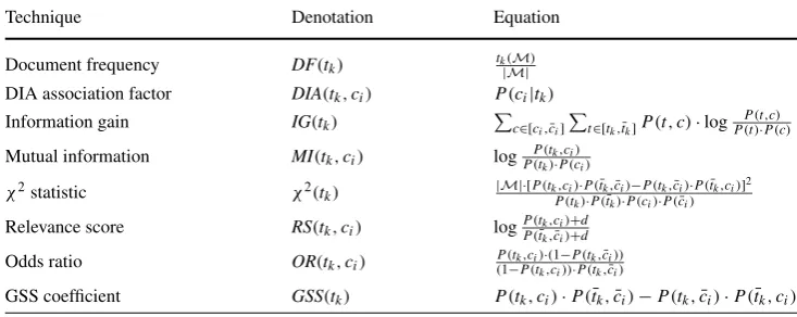
Table 1 The most popular
term-selection techniques Technique Denotation Equation
Document frequency DF(tk) tk|(MM|)
DIA association factor DIA(tk, ci) P (ci|tk)
Information gain IG(tk) c∈[ci,c¯i]
t∈[tk,¯tk]P (t, c)·log P (t,c) P (t )·P (c)
Mutual information MI(tk, ci) logP (tP (tk)k·P (c,ci)i)
χ2statistic χ2(tk) |M|·[P (tk,ci)·P (¯tk,¯ci)−P (tk,¯ci)·P (¯tk,ci)] 2 P (tk)·P (¯tk)·P (ci)·P (¯ci)
Relevance score RS(tk, ci) logP (tP (¯tkk,¯,ccii)+d)+d
Odds ratio OR(tk, ci) (P (t1−P (tk,ci)·(k,c1i−P (t))·P (tkk,c,¯¯ci))i)
GSS coefficient GSS(tk) P (tk, ci)·P (t¯k,c¯i)−P (tk,c¯i)·P (t¯k, ci)
3.2.8 GSS coefficient
GSS coefficient is a simplified variant of χ2 statistic pro-posed by Galavotti et al. [24], which is defined as
GSS(tk)=P (tk, ci)·P
¯
tk,c¯i
−Ptk,c¯i
·Pt¯k, ci
.
The greater (smaller) the positive (negative) values, the stronger the terms tk will be to indicate the membership
(non-membership) of classci.
For convenience, the mathematical equations of all pre-sented techniques are summarized in Table1.5
4 Naive Bayes spam filters
Probabilistic classifiers are historically the first proposed fil-ters. These approaches are the most employed in propri-etary and open-source systems proposed for spam filtering because of their simplicity and high performance [35,38,
46].
Given a set of messages M = {m1, m2, . . . , mj, . . . ,
m|M|} and category set C = {spam(cs), legitimate(cl)},
wheremj is thejth mail inMandCis the possible label
set, the task of automated spam filtering consists in build-ing a Boolean categorization functionΦ(mj, ci):M×C→
{True,False}. WhenΦ(mj, ci)isTrue, it indicates that
messagemj belongs to categoryci; otherwise,mj does not
belong toci.
In the setting of spam filtering there exist only two cate-gory labels:spamandlegitimate. Each messagemj∈
M can only be assigned to one of them, but not to both. Therefore, we can use a simplified categorization function Φspam(mj):M→ {True,False}. Hence, a message is
classified as spam whenΦspam(mj)isTrue, and legitimate
otherwise.
5Table1shows all term-selection techniques presented in this section in terms of subjective probability. The equations refer to the “local” forms of the functions.
The application of supervised machine learning algo-rithms for spam filtering consists of two stages:
1. Training. A set of labeled messages (M) must be pro-vided as training data, which are first transformed into a representation that can be understood by the learning algorithms. The most commonly used representation for spam filtering is the vector space model, in which each documentmj∈Mis transformed into a real vectorxj∈
|S|, whereSis the vocabulary (feature set) and the
co-ordinates ofxj represent the weight of each feature inS.
Then, we can run a learning algorithm over the training data to create a classifierΦspam(xj)→ {True,False}. 2. Classification. The classifierΦspam(xj)is applied to the vector representation of a messagexto produce a predic-tion whetherxis spam or not.
From Bayes’ theorem and the theorem of the total prob-ability, the probability that a message with vector x = x1, . . . , xnbelongs to a categoryci∈ {cs, cl}is:
P (ci|x)=
P (ci)·P (x|ci)
P (x) .
Since the denominator does not depend on the category, Naive Bayes (NB) filter classifies each message in the cat-egory that maximizesP (ci)·P (x|ci). In the spam filtering
domain it is equivalent to classify a message as spam (cs)
whenever
P (cs)·P (x|cs)
P (cs)·P (x|cs)+P (cl)·P (x|cl)
> T ,
withT =0.5. By varyingT, we can opt for more true neg-atives (legitimate messages correctly classified) at the ex-pense of fewer true positives (spam messages correctly clas-sified), or vice versa. Thea prioriprobabilitiesP (ci)can
be estimated as frequency of occurrences of documents be-longing to the category ci in the training set M, whereas
P (x|ci) is practically impossible to estimate directly
a simple assumption that the terms in a message are condi-tionally independent and the order they appear is irrelevant. The probabilitiesP (x|ci)are estimated differently in each
NB model.
Despite the fact that its independence assumption is usu-ally over-simplistic, several studies have found the NB clas-sifier to be surprisingly effective in the spam filtering task [7,35].
In the following, we describe the seven most studied models of NB spam filter available in the literature. 4.1 Basic Naive Bayes
We call Basic NB the first NB spam filter proposed by Sa-hami et al. [40]. LetS= {t1, . . . , tn}be the set of terms after
the term selection; each messagemis represented as a bi-nary vectorx= x1, . . . , xn, where eachxk shows whether
or nottk will occur inm. The probabilitiesP (x|ci)are
cal-culated by
P (x|ci)= n
k=1
P (tk|ci),
and the criterion for classifying a message as spam is P (cs)·
n
k=1P (tk|cs)
ci∈{cs,cl}P (ci)·
n
k=1P (tk|ci)
> T .
Here, probabilitiesP (tk|ci)are estimated by
P (tk|ci)=|Mtk,ci|
|Mci|
,
where|Mtk,ci|is the number of training messages of cate-goryci that contain the termtk, and|Mci|is the total num-ber of training messages that belong to the categoryci.
4.2 Multinomial term frequency Naive Bayes
The multinomial term frequency NB (MN TF NB) repre-sents each message as a set of termsm= {t1, . . . , tn},
com-puting each one oftkas many times as it appears inm. In this
sense, mcan be represented by a vectorx= x1, . . . , xn,
where eachxkcorresponds to the number of occurrences of
tk inm. Moreover, each messagemof categoryci can be
interpreted as the result of picking independently|m|terms fromSwith replacement and probabilityP (tk|ci)for each
tk [37]. Hence,P (x|ci)is the multinomial distribution:
P (x|ci)=P (|m|)· |m|! · n
k=1
P (tk|ci)xk
xk!
.
Thus, the criterion for classifying a message as spam be-comes
P (cs)·
n
k=1P (tk|cs)xk
ci∈{cs,cl}P (ci)·
n
k=1P (tk|ci)xk
> T ,
and the probabilitiesP (tk|ci)are estimated as a Laplacian
prior
P (tk|ci)=
1+Ntk,ci
n+Nci
,
whereNtk,ci is the number of occurrences of termtk in the training messages of categoryci, andNci=
n
k=iNtk,ci. 4.3 Multinomial Boolean Naive Bayes
The multinomial Boolean NB (MN Boolean NB) is simi-lar to the MN TF NB, including the estimates ofP (tk|ci),
except that each attribute xk is Boolean. Note that these
approaches do not take into account the absence of terms (xk=0) from the messages.
Schneider [43] demonstrates that MN Boolean NB may perform better than MN TF NB. This is because the multino-mial NB with term frequency attributes is equivalent to an NB version with the attributes modeled as following Poisson distributions in each category, assuming that the message length is independent of the category. Therefore, the multinomial NB may achieve better performance with Boolean attributes if the term frequencies attributes do not follow Poisson distributions.
4.4 Multivariate Bernoulli Naive Bayes
LetS= {t1, . . . , tn}be the result set of terms after the term
selection. The multivariate Bernoulli NB (MV Bernoulli NB) represents each messagemby computing the presence and absence of each term. Therefore,mcan be represented as a binary vector x= x1, . . . , xn, where eachxk shows
whether or nottk will occur inm. Moreover, each message
mof categoryci is seen as the result ofnBernoulli trials,
where at each trial we decide whether or not tk will
ap-pear inm. The probability of a positive outcome at trialk isP (tk|ci). Then, the probabilitiesP (x|ci)are computed by
P (x|ci)= n
k=1
P (tk|ci)xk·
1−P (tk|ci)
(1−xk).
The criterion for classifying a message as spam becomes
P (cs)·
n
k=1P (tk|cs)xk·(1−P (tk|cs))(1−xk)
ci∈{cs,cl}P (ci)·
n
k=1P (tk|ci)xk·(1−P (tk|ci))(1−xk) > T ,
and probabilities P (tk|ci) are estimated as a Laplacian
prior
P (tk|ci)=
1+ |Mtk,ci| 2+ |Mci|
,
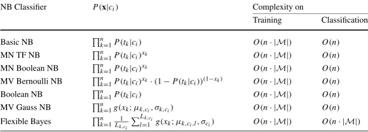
Table 2 Naive Bayes spam
filters NB Classifier P (x|ci) Complexity on
Training Classification
Basic NB nk=1P (tk|ci) O(n· |M|) O(n)
MN TF NB nk=1P (tk|ci)xk O(n· |M|) O(n)
MN Boolean NB nk=1P (tk|ci)xk O(n· |M|) O(n)
MV Bernoulli NB nk=1P (tk|ci)xk·(1−P (tk|ci))(1−xk) O(n· |M|) O(n)
Boolean NB nk=1P (tk|ci) O(n· |M|) O(n)
MV Gauss NB nk=1g(xk;μk,ci, σk,ci) O(n· |M|) O(n)
Flexible Bayes nk=1L1
k,ci Lk,ci
l=1 g(xk;μk,ci,l, σci) O(n· |M|) O(n· |M|)
number of training messages of categoryci. For more
the-oretical explanation, consult Metsis et al. [38] and Losada and Azzopardi [34].
4.5 Boolean Naive Bayes
We denote as Boolean NB the classifier similar to the MV Bernoulli NB with the difference that it does not take into ac-count the absence of terms. Hence, the probabilitiesP (x|ci)
are estimated only by
P (x|ci)= n
k=1
P (tk|ci),
and the criterion for classifying a message as spam becomes
P (cs)·
n
k=1P (tk|cs)
ci∈{cs,cl}P (ci)·
n
k=1P (tk|ci)
> T ,
where probabilitiesP (tk|ci)are estimated in the same way
as used in the MV Bernoulli NB.
4.6 Multivariate Gauss Naive Bayes
Multivariate Gauss NB (MV Gauss NB) uses real-valued at-tributes by assuming that each attribute follows a Gaussian distribution g(xk;μk,ci, σk,ci) for each category ci, where the μk,ci andσk,ci of each distribution are estimated from the training setM.
The probabilitiesP (x|ci)are calculated by
P (x|ci)= n
k=1
g(xk;μk,ci, σk,ci),
and the criterion for classifying a message as spam becomes P (cs)·
n
k=1g(xk;μk,cs, σk,cs)
ci∈{cs,cl}P (ci)·
n
k=1g(xk;μk,ci, σk,ci)
> T .
4.7 Flexible Bayes
Flexible Bayes (FB) works similarly to MV Gauss NB. However, instead of using a single normal distribution for each attributeXk per categoryci, FB represents the
proba-bilitiesP (x|ci)as the average ofLk,ci normal distributions with different values forμk,cibut the same one forσk,ci:
P (xk|ci)=
1 Lk,ci
Lk,ci
l=1
g(xk;μk,ci,l, σci),
whereLk,ci is the quantity of different values that the at-tributeXk has in the training setMof categoryci. Each of
these values is used asμk,ci,lof a normal distribution of the categoryci. However, all distributions of a categoryci are
taken to have the sameσci= 1 √
|Mci| .
The distribution of each category becomes narrower as more training messages of that category are accumulated. By averaging several normal distributions, FB can approx-imate the true distributions of real-valued attributes more closely than the MV Gauss NB when the assumption that attributes follow normal distribution is violated. For further details, consult John and Langley [28] and Androutsopoulos et al. [7].
Table2summarizes all NB spam filters presented in this section.6
5 Performance measurements
According to Cormack [14], the filters should be judged along four dimensions: autonomy, immediacy, spam identi-fication, and non-spam identification. However, it is not ob-vious how to measure any of these dimensions separately, nor how to combine these measurements into a single one for the purpose of comparing filters. Reasonable standard
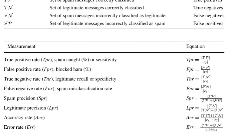
Table 3 All possible prediction
results Notation Composition Also known as
T P Set of spam messages correctly classified True positives
T N Set of legitimate messages correctly classified True negatives
FN Set of spam messages incorrectly classified as legitimate False negatives
FP Set of legitimate messages incorrectly classified as spam False positives
Table 4 Popular performance measurements used in the literature
Measurement Equation
True positive rate (Tpr), spam caught (%) or sensitivity Tpr=|T P|c |
s|
False positive rate (Fpr), blocked ham (%) Fpr=|FP|c |
l|
True negative rate (Tnr), legitimate recall or specificity Tnr=|T N|c |
l|
False negative rate (Fnr), spam misclassification rate Fnr=|FN|c |
s|
Spam precision (Spr) Spr=|T P|T P|+|FP| |
Legitimate precision (Lpr) Lpr=|T N|T N|+|FN| |
Accuracy rate (Acc) Acc=|T P|c|+|T N|
s|+|cl|
Error rate (Err) Err=|FP|c|+|FN|
s|+|cl|
measures are useful to facilitate comparison, given that the goal of optimizing them does not replace that of finding the most suitable filter for the purpose of spam filtering.
Considering the category set C = {spam(cs),
legitimate(cl)}and all possible prediction results presented
in Table 3, some well-known evaluation measures are pre-sented in Table4.
All the measures presented in Table 4 consider a false negative as harmful as a false positive. Nevertheless, failures to identify legitimate and spam messages have different con-sequences [14,15]. According to Cormack [14], misclassi-fied legitimate messages increase the risk that the informa-tion contained in the message will be lost, or at least de-layed. It is very difficult to measure the amount of risk and delay that can be supported, once the consequences depend on the relevance of the message content for a given user. On the other hand, failures to identify spam also vary in impor-tance, but are generally less critical than failures to identify non-spam. Viruses, worms, and phishing messages may be an exception, as they pose significant risks to the user.
Whatever the measure adopted, an aspect to be consid-ered is the asymmetry in the misclassification costs. A spam message incorrectly classified as legitimate is a significantly minor problem, as the user is simply required to remove it. On the other hand, a legitimate message mislabeled as spam can be unacceptable, as it implies the loss of potentially im-portant information, particularly for those settings in which spam messages are automatically deleted.
To overcome the lack of symmetry, Androutsopoulos et al. [5] proposed a further refinement based on spam recall and precision in order to allow the performance evaluation
based on a single measure. They consider a false positive as beingλtimes more costly than false negatives, whereλ equals to 1 or 9. Thus, each false positive is accounted asλ mistakes.
In this case, the total cost ratio (TCR) can be calculated by
TCR= |cs| λ|FP| + |FN|.
TCRis an evaluation measurement commonly employed to compare the performances achieved by different spam fil-ters. It offers an indication of the improvement provided by the filter. A biggerTCRindicates a better performance, and forTCR<1, not using the filter is preferable.
The problem of using TCR is that it does not return a value inside a predefined range [10,15]. For instance, con-sider two classifiersAandB employed to filter 600 mes-sages (450 spams+150 legitimates,λ=1). Suppose that Aattains a perfect prediction withFPA=FNA=0, and
Bincorrectly classifies 3 spam messages as legitimate, thus FPB=0 andFNB=3.
In this way,TCRA= +∞andTCRB=150. Intuitively,
To avoid those drawbacks, we propose the use of the Matthews correlation coefficient (MCC) [36] for assessing the performance of spam classifiers. MCC is used in ma-chine learning as a quality measure of binary classifications, which provides much more information thanTCR. It returns a real value between−1 and+1. A coefficient equal to+1 indicates a perfect prediction; 0, an average random predic-tion; and−1, an inverse prediction.
MCC provides a balanced evaluation of the prediction (i.e., the proportion of correct predictions for each class), especially if the two classes are of very different sizes [8]. It can be calculated by
MCC=√ (|T P| · |T N|)−(|FP| · |FN|)
(|T P| + |FP|)·(|T P| + |FN|)·(|T N| + |FP|)·(|T N| + |FN|). Using the previous example, the classifiers A and B achieve MCCA=1.000 andMCCB=0.987, respectively.
Now, it is noteworthy that we can make correct assumptions for the prediction in-between the classifiers as well as for each individual performance.
As with TCR, we can define an independent rateλ >1 to indicate how much a false positive is worse than a false negative. For that, the amount of false positives (|FP|) in theMCCequation is simply multiplied byλ:
MCC= (|T P| · |T N|)−(λ|FP| · |FN|)
(|T P| +λ|FP|)·(|T P| + |FN|)·(|T N| +λ|FP|)·(|T N| + |FN|).
Moreover,MCC can also be combined with other mea-sures in order to guarantee a fairer comparison, such as precision×recall, blocked hams (false positive) and spam caught (true positive) rates.
6 Experimental protocol
In this section, we present the experimental protocol de-signed for the empirical evaluation of the different term-selection methods presented in Sect. 3. They were applied for reducing the dimensionality of the term space before the classification task performed by the Bayesian filters pre-sented in Sect.4.
We carried out this study on the six well-known, large, real and public Enron7data sets. The corpora are composed of legitimate messages extracted from the mailboxes of six former employees of the Enron Corporation. For further de-tails about the data set statistics and composition, refer to Metsis et al. [38].
For providing an aggressive dimensionality reduction, we performed the training stage using the first 90% of the re-ceived messages (training set). The remaining ones were separated for classifying (testing set).
7The Enron data sets are available at http://www.iit.demokritos.gr/ skel/i-config/.
After the training stage, we applied the term-selection techniques (TSTs) presented in Sect.3for reducing the di-mensionality of the term space.8In order to perform a com-prehensive performance evaluation, we varied the number of terms to be selected from 10 to 100% of all retained terms in the preprocessing stage.
Next, we classified the testing messages using the Naive Bayes spam filters presented in Sect.4. We set the classifica-tion thresholdT =0.5 (λ=1) as used in Metsis et al. [38]. By varyingT, we can opt for more true negatives at the cost of fewer true positives, or vice versa.
We tested all possible combinations between NB spam filters and term-selection methods. In spite of using all the performance measurements presented in Table4for evalu-ating the classifiers, we selected theMCCto compare their results.
7 Experimental results
This section presents the results achieved for each corpus. In the remainder of this paper, consider the following abbrevi-ations: Basic NB as Bas, Boolean NB as Bool, MN Boolean NB as MN Bool, MN term frequency NB as MN TF, MV Bernoulli NB as Bern, MV Gauss NB as Gauss, and flexible Bayes as FB.
7.1 Overall analysis
Due to space limitations, we present only the best combi-nation (i.e., TST and % of|S|) for each NB classifier.9We define “best result” the combination that obtained the high-estMCC.
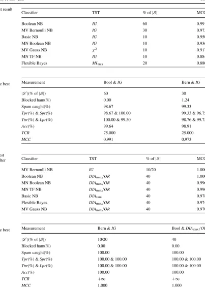
Tables5,7,9,11,13, and15show the best combination for each filter and its correspondingMCC. Additionally, we present the complete set of performance measures for the best classifiers in Tables6,8,10,12,14, and16.
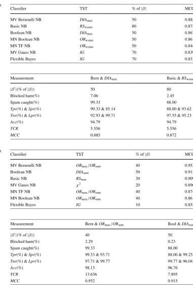
It can be seen from Table6that both Bern withDIAmax @50% and Basic with RSwsum@80% obtained the same TCRbut differentMCCfor Enron 1. This happens because theMCCoffers a balanced evaluation of the prediction, par-ticularly if the classes are of different sizes, as discussed in Sect.5.
Table 11 shows another drawback of TCR. Bern with IG@10% achieved a perfect prediction (|FP| = |FN| =0) for Enron 4, attainingMCC=1.000 and TCR= +∞. On the other hand, Bool withDIAmax@40% incorrectly classi-fied one spam as legitimate (|FP| =0,|FN| =1), accom-plishingMCC=0.996 andTCR=450. If we analyze only
Table 5 Enron 1: the best result
achieved by each NB filter Classifier TST % of|S| MCC
MV Bernoulli NB DIAmax 50 0.885
Basic NB RSwsum 80 0.872
Boolean NB DIAmax 50 0.867
MN Boolean NB ORwsum 50 0.861
MN TF NB ORwsum 50 0.844
MV Gauss NB IG 70 0.839
Flexible Bayes IG 70 0.833
Table 6 Enron 1: two classifiers that attained the best individual performance
Measurement Bern &DIAmax Basic &RSwsum
|S|(% of|S|) 50 80
Blocked ham(%) 7.06 2.45
Spam caught(%) 99.33 88.00
Tpr(%) &Spr(%) 99.33 & 85.14 88.00 & 93.62 Tnr(%) &Lpr(%) 92.93 & 99.71 97.55 & 95.23
Acc(%) 94.79 94.79
TCR 5.556 5.556
MCC 0.885 0.872
Table 7 Enron 2: the best result
achieved by each filter Classifier TST % of|S| MCC
MV Bernoulli NB ORmax/ORsum 40 0.952
Boolean NB DIAsum 50 0.915
Basic NB RSmax 30 0.909
MV Gauss NB χ2 20 0.896
MN TF NB ORmax/ORsum 40 0.874
MN Boolean NB ORmax/ORsum 40 0.861
Flexible Bayes IG 10 0.855
Table 8 Enron 2: two classifiers that attained the best individual performance
Measurement Bern &ORmax/ORsum Bool &DIAsum
|S|(% of|S|) 40 50
Blocked ham(%) 2.29 0.23
Spam caught(%) 99.33 88.00
Tpr(%) &Spr(%) 99.33 & 93.71 88.00 & 99.25 Tnr(%) &Lpr(%) 97.71 & 99.77 99.77 & 96.04
Acc(%) 98.13 96.76
TCR 13.636 7.895
MCC 0.952 0.915
theTCR, we may wrongly claim that the first combination is much better than the second one.
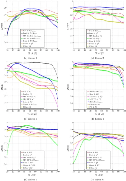
Figure1 shows the TSTs that attained the best average prediction (i.e., the highest area under the curve) for each NB classifier. In this figure, we present the individual results of each data set.
Table 9 Enron 3: the best result
achieved by each filter Classifier TST % of|S| MCC
Boolean NB IG 60 0.991
MV Bernoulli NB IG 30 0.973
Basic NB IG 10 0.950
MN Boolean NB IG 10 0.936
MV Gauss NB χ2 10 0.917
MN TF NB IG 10 0.884
Flexible Bayes MImax 20 0.880
Table 10 Enron 3: two classifiers that attained the best individual performance
Measurement Bool &IG Bern &IG
|S|(% of|S|) 60 30
Blocked ham(%) 0.00 1.24
Spam caught(%) 98.67 99.33
Tpr(%) &Spr(%) 98.67 & 100.00 99.33 & 96.75 Tnr(%) &Lpr(%) 100.00 & 99.50 98.76 & 99.75
Acc(%) 99.64 98.91
TCR 75.000 25.000
MCC 0.991 0.973
Table 11 Enron 4: the best
result achieved by each filter Classifier TST % of|S| MCC
MV Bernoulli NB IG 10/20 1.000
Boolean NB DIAmax/OR 40 1.000
MN Boolean NB DIAmax/OR 40 0.996
MN TF NB DIAmax/OR 40 0.996
Basic NB DIAsum 40 0.978
Flexible Bayes DIAmax/OR 40 0.974
MV Gauss NB DIAmax/OR 40 0.970
Table 12 Enron 4: two classifiers that attained the best individual performance
Measurement Bern &IG Bool &DIAmax/OR
|S|(% of|S|) 10/20 40
Blocked ham(%) 0.00 0.00
Spam caught(%) 100.00 100.00
Tpr(%) &Spr(%) 100.00 & 100.00 100.00 & 100.00 Tnr(%) &Lpr(%) 100.00 & 100.00 100.00 & 100.00
Acc(%) 100.00 100.00
TCR +∞ +∞
MCC 1.000 1.000
all the terms ofS. On the other hand, it is also noteworthy that MI often achieves better results when we employ the complete set of terms|S|.
Regarding the TSTs, the results indicate that{IG, χ2,DF, OR,DIA}>{RS,GSS} MI, where “>” means “performs better than.” However, if we consider the average prediction,
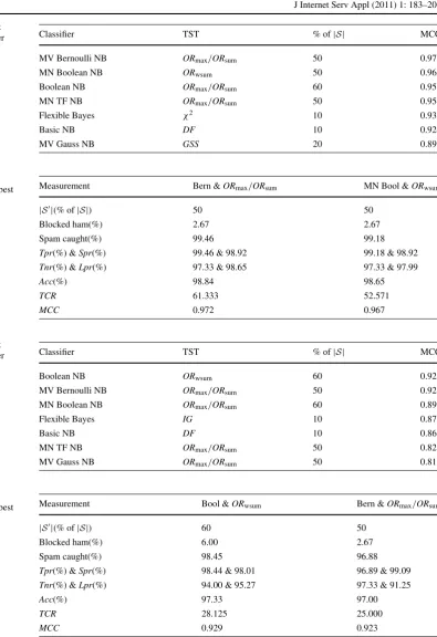
Table 13 Enron 5: the best
result achieved by each filter Classifier TST % of|S| MCC
MV Bernoulli NB ORmax/ORsum 50 0.972
MN Boolean NB ORwsum 50 0.967
Boolean NB ORmax/ORsum 60 0.955
MN TF NB ORmax/ORsum 50 0.954
Flexible Bayes χ2 10 0.931
Basic NB DF 10 0.924
MV Gauss NB GSS 20 0.895
Table 14 Enron 5: two classifiers that attained the best individual performance
Measurement Bern &ORmax/ORsum MN Bool &ORwsum
|S|(% of|S|) 50 50
Blocked ham(%) 2.67 2.67
Spam caught(%) 99.46 99.18
Tpr(%) &Spr(%) 99.46 & 98.92 99.18 & 98.92 Tnr(%) &Lpr(%) 97.33 & 98.65 97.33 & 97.99
Acc(%) 98.84 98.65
TCR 61.333 52.571
MCC 0.972 0.967
Table 15 Enron 6: the best
result achieved by each filter Classifier TST % of|S| MCC
Boolean NB ORwsum 60 0.929
MV Bernoulli NB ORmax/ORsum 50 0.923
MN Boolean NB ORmax/ORsum 60 0.897
Flexible Bayes IG 10 0.873
Basic NB DF 10 0.866
MN TF NB ORmax/ORsum 50 0.829
MV Gauss NB ORmax/ORsum 50 0.819
Table 16 Enron 6: two classifiers that attained the best individual performance
Measurement Bool &ORwsum Bern &ORmax/ORsum
|S|(% of|S|) 60 50
Blocked ham(%) 6.00 2.67
Spam caught(%) 98.45 96.88
Tpr(%) &Spr(%) 98.44 & 98.01 96.89 & 99.09 Tnr(%) &Lpr(%) 94.00 & 95.27 97.33 & 91.25
Acc(%) 97.33 97.00
TCR 28.125 25.000
MCC 0.929 0.923
1.000) for Enron 4 when we use 10% of |S| selected by IG, whereas it attainedMCC= −0.082 when we em-ployMIsum.
With respect to the filters, the individual and average re-sults indicate that {Boolean NB, MV Bernoulli NB, Basic NB} > {MN Boolean NB, MN term frequency NB} >
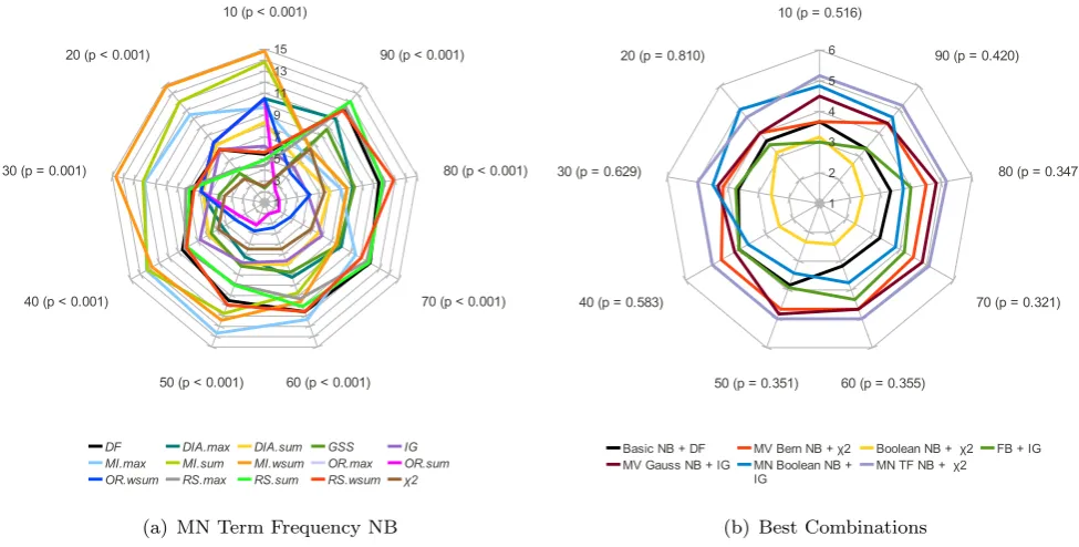
Fig. 3 Average rank achieved by TSTs for MN Term Frequency NB spam filter (a) and the best combinations between filters and TSTs (b)
Table 17 Summary of the
observed results Classifier % of|S| Highlights
Best Worst
Basic NB 10–30 DF,GSS,RS,χ2 MI
MV Bernoulli NB 10–20 χ2,GSS,RS,DF MI
MV Bernoulli NB 70 OR DIAmax,MI
Boolean NB 10–70 χ2 MI
Flexible Bayes 10–70 IG DIAsum,MI
MV Gauss NB 10–40 IG,χ2,GSS MI
MN Boolean NB 10–80 IG MI
MN Term Frequency NB 10–50 χ2 MI
MN Term Frequency NB 50–100 OR DF,RS
users generally receive messages with some specific terms, such as names or signatures.
7.2 Statistical analysis
In the following, we present a statistical analysis of the re-sults. For that, we used a Friedman’s test [17] for compar-ing the distribution of ranks among the analyzed algorithms across the six Enron data sets.
Figures 2 and3(a) show the average rank achieved by each TST.10 In those figures, we present the individual re-sults of each spam classifier. Thex axis shows the different
10All color pictures are available at http://www.dt.fee.unicamp.br/ ~tiago/Research/Spam/spam.htm.
values of|S|% and thep-values at each level. It is impor-tant to note that the smaller the geometric area, the better the technique. According to Nemenyi test [17], the critical distance (CD) for pairwise comparisons between TSTs at p=0.01 is 8.16.
Table17summarizes the analysis of the results. For each classifier, we present the % of|S|in which we observe sta-tistical differences between the TSTs. In those cases, we identify three groups. Clearly, the best methods outperform the worst ones. However, the experimental data are not suf-ficient for assuming any conclusion to which group the re-mainder of techniques belong.
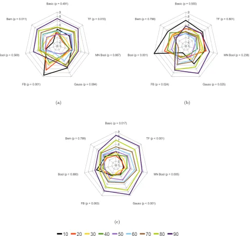
Fig. 4 Average rank achieved by NB filters when document frequency (a), information gain (b) andχ2statistic (c) are used
When |S|% varies from 10 to 30%, there is a significant statistical difference between TSTs. Notice that the perfor-mance of MIsum and MIwsum is significantly worse than that ofDF,GSS,RSandχ2for such an interval. However, we cannot reach any conclusion regarding the remainder of TSTs.
Another interesting result can be observed in Fig. 2(d). IGundoubtedly achieved the best average rank for Flexible Bayes. MI has attained again the worst average rank. The performance of MIsum and MIwsum is significantly worse thanIGwhen 10–70% of|S|was selected.
Additionally, we have compared the average rank at-tained by the statistically best combinations (NB spam filter
and TST), as illustrated in Fig.3(b). Although the results in-dicate that Boolean NB withχ2statistic is better (in average rank) than any other evaluated combination, the experimen-tal data is not sufficient to reach any conclusion.
Finally, we have also evaluated how the number of se-lected terms affects the average rank achieved by the statis-tically best TSTs (DF,IGandχ2statistic) for all the com-pared NB spam filters (Fig.4).
In general, the statistical results are consistent with the in-dividual best results (Sect.7.1), with few exceptions. For in-stance, MV Bernoulli NB has presented good individual per-formance for each e-mail collection and, however, the statis-tical analysis indicates that such a filter is inferior to Basic NB and Boolean NB in average rank. Moreover, the Fried-man’s test also indicates that Flexible Bayes is not worse than other filters, as the individual results have presented.
8 Conclusions and further work
In this paper, we have presented a performance evaluation of several term-selection methods in dimensionality reduc-tion for the spam filtering domain by classifiers based on the Bayesian decision theory. We have performed the compar-ison of the performance achieved by seven different Naive Bayes spam filters applied to classify messages from six well-known, real, public and large e-mail data sets, after a step of dimensionality reduction employed by eight popu-lar term-selection techniques varying the number of selected terms.
Furthermore, we have proposed the Matthews correla-tion coefficient (MCC) as the evaluacorrela-tion measure instead of the total cost ratio (TCR).MCC provides a more balanced evaluation of the prediction thanTCR, especially if the two classes are of different sizes. Moreover, it returns a value in-side a predefined range, which provides more information about the classifiers’ performance.
Regarding term-selection techniques, we have found that DF,IG, andχ2statistic are the most effective in aggressive term removal without losing categorization accuracy. DIA, RS,GSS coefficient andORalso provide an improvement on the filters’ performance. On the other hand,MIgenerally offers poor results which frequently worsen the classifiers’ performance.
Among of all presented classifiers, Boolean NB and Ba-sic NB achieved best individual and average rank perfor-mance. The results also verify that Boolean attributes per-form better than the term frequency ones as presented by Schneider [43].
We also have shown that the performance of Naive Bayes spam classifiers is highly sensitive to the selected attributes and the number of selected terms by the term-selection methods in the training stage. The better the term-selection technique, the better the filters’ prediction.
Future works should take into consideration that spam fil-tering is a co-evolutionary problem, because while the filter tries to evolve its prediction capacity, the spammers try to evolve their spam messages in order to overreach the classi-fiers. Hence, an efficient approach should have an effective way to adjust its rules in order to detect the changes of spam features. In this way, collaborative filters [33] could be used
to assist the classifier by accelerating the adaptation of the rules and increasing the classifiers’ performance. Moreover, spammers generally insert a large amount of noise in spam messages in order to make the probability estimation more difficult. Thus, the filters should have a flexible way to com-pare the terms in the classifying task. Approaches based on fuzzy logic [49] could be employed to make the comparison and selection of terms more flexible.
Acknowledgement This work is partially supported by the Brazilian funding agencies CNPq, CAPES and FAPESP.
References
1. Almeida T, Yamakami A (2010) Content-based spam filtering. In: Proceedings of the 23rd IEEE international joint conference on neural networks, Spain, Barcelona, pp 1–7
2. Almeida T, Yamakami A, Almeida J (2009) Evaluation of ap-proaches for dimensionality reduction applied with Naive Bayes anti-spam filters. In: Proceedings of the 8th IEEE international conference on machine learning and applications, Miami, FL, USA, pp 517–522
3. Almeida T, Yamakami A, Almeida J (2010) Filtering spams using the minimum description length principle. In: Proceedings of the 25th ACM symposium on applied computing, Sierre, Switzerland, pp 1856–1860
4. Almeida T, Yamakami A, Almeida J (2010) Probabilistic anti-spam filtering with dimensionality reduction. In: Proceedings of the 25th ACM symposium on applied computing, Sierre, Switzer-land, pp 1802–1806
5. Androutsopoulos I, Koutsias J, Chandrinos K, Paliouras G, Spy-ropoulos C (2000) An evaluation of Naive Bayesian anti-spam fil-tering. In: Proceedings of the 11st European conference on ma-chine learning, Barcelona, Spain, pp 9–17
6. Androutsopoulos I, Paliouras G, Karkaletsis V, Sakkis G, Spy-ropoulos C, Stamatopoulos P (2000) Learning to filter spam e-mail: a comparison of a Naive Bayesian and a memory-based approach. In: Proceedings of the 4th European conference on prin-ciples and practice of knowledge discovery in databases, Lyon, France, pp 1–13
7. Androutsopoulos I, Paliouras G, Michelakis E (2004) Learning to filter unsolicited commercial e-mail. Technical Report 2004/2, National Centre for Scientific, Research “Demokritos”, Athens, Greece
8. Baldi P, Brunak S, Chauvin Y, Andersen C, Nielsen H (2000) As-sessing the accuracy of prediction algorithms for classification: an overview. Bioinformatics 16(5):412–424
9. Bratko A, Cormack G, Filipic B, Lynam T, Zupan B (2006) Spam filtering using statistical data compression models. J Mach Learn Res 7:2673–2698
10. Carpinter J, Hunt R (2006) Tightening the Net: a review of current and next generation spam filtering tools. Comput Secur 25(8):566–578
11. Carreras X, Marquez L (2001) Boosting trees for anti-spam email filtering. In: Proceedings of the 4th international conference on re-cent advances in natural language processing, Tzigov Chark, Bul-garia, pp 58–64
12. Cohen W (1995) Fast effective rule induction. In: Proceedings of 12nd international conference on machine learning, Tahoe City, CA, USA, pp 115–123
14. Cormack G (2008) Email spam filtering: a systematic review. Found Trends Inf Retr 1(4):335–455
15. Cormack G, Lynam T (2007) Online supervised spam filter evalu-ation. ACM Trans Inf Syst 25(3):1–11
16. Cunningham P, Nowlan N, Delany S, Haahr M (2003) A case-based approach to spam filtering that can track concept drift. In: Proceedings of the 5th international conference on case based rea-soning. Trondheim, Norway, pp 115–123
17. Demsar J (2006) Statistical comparisons of classifiers over multi-ple data sets. J Mach Learn Res 7:1–30
18. Drucker H, Wu D, Vapnik V (1999) Support vector machines for spam categorization. IEEE Trans Neural Netw 10(5):1048–1054 19. Forman G (2003) An extensive empirical study of feature selection
metrics for text classification. J Mach Learn Res 3:1289–1305 20. Forman G, Kirshenbaum E (2008) Extremely fast text feature
ex-traction for classification and indexing. In: Proceedings of 17th ACM conference on information and knowledge management, Napa Valley, CA, USA, pp 1221–1230
21. Forman G, Scholz M, Rajaram S (2000) Feature shaping for lin-ear SVM classifiers. In: Proceedings of the 15th ACM SIGKDD international conference on knowledge discovery and data mining. Paris, France, pp 299–308
22. Friedman N, Geiger D, Goldszmidt M (1997) Bayesian network classifiers. Mach Learn 29(3):131–163
23. Fuhr N, Buckley C (1991) A probabilistic learning approach for document indexing. ACM Trans Inf Syst 9(3):223–248
24. Galavotti L, Sebastiani F, Simi M (2000) Experiments on the use of feature selection and negative evidence in automated text cat-egorization. In: Proceedings of 4th European conference on re-search and advanced technology for digital libraries, Lisbon, Por-tugal, pp 59–68
25. Guzella T, Caminhas W (2000) A review of machine learning ap-proaches to spam filtering. Exp Syst Appl 36(7):10206–10222 26. Hidalgo J (2002) Evaluating cost-sensitive unsolicited bulk email
categorization. In: Proceedings of the 17th ACM symposium on applied computing, Madrid, Spain, pp 615–620
27. Joachims T (1997) A probabilistic analysis of the Rocchio al-gorithm with TFIDF for text categorization. In: Proceedings of 14th international conference on machine learning, Nashville, TN, USA, pp 143–151
28. John G, Langley P (1995) Estimating continuous distributions in Bayesian classifiers. In: Proceedings of the 11st international con-ference on uncertainty in artificial intelligence, Montreal, Canada, pp 338–345
29. John G, Kohavi R, Pfleger K (1994) Irrelevant features and the subset selection problem. In: Proceedings of 11st international conference on machine learning, New Brunswick, NJ, USA, pp 121–129
30. Kira K, Rendell L (1992) A practical approach to feature selec-tion. In: Proceedings of the 9th international workshop on machine learning, Aberdeen, Scotland, UK, pp 249–256
31. Kolcz A, Alspector J (2001) SVM-based filtering of e-mail spam with content-specific misclassification costs. In: Proceedings of the 1st international conference on data mining, San Jose, CA, USA, pp 1–14
32. Koprinska I, Poon J, Clark J, Chan J (2007) Learning to classify e-mail. Inf Sci 177(10):2167–2187
33. Lemire D (2005) Scale and translation invariant collaborative fil-tering systems. Inf Retr 8(1):129–150
34. Losada D, Azzopardi L (2008) Assessing multivariate Bernoulli models for information retrieval. ACM Trans Inf Syst 26(3):1–46 35. Marsono M, El-Kharashi N, Gebali F (2009) Targeting spam
trol on middleboxes: spam detection based on layer-3 e-mail con-tent classification. Comput Netw 53(6):835–848
36. Matthews B (1975) Comparison of the predicted and observed sec-ondary structure ofT4phage lysozyme. Biochim Biophys Acta 405(2):442–451
37. McCallum A, Nigam K (1998) A comparison of event models for Naive Bayes text classification. In: Proceedings of the 15th AAAI workshop on learning for text categorization, Menlo Park, CA, USA, pp 41–48
38. Metsis V, Androutsopoulos I, Paliouras G (2006) Spam filtering with Naive Bayes—which Naive Bayes. In: Proceedings of the 3rd international conference on email and anti-spam, Mountain View, CA, USA, pp 1–5
39. Mitchell T (1997) Machine learning. McCraw-Hill, New York 40. Sahami M, Dumais S, Hecherman D, Horvitz E (1998) A Bayesian
approach to filtering junk e-mail. In: Proceedings of the 15th na-tional conference on artificial intelligence, Madison, WI, USA, pp 55–62
41. Schapire R, Singer Y, Singhal A (1998) Boosting and Rocchio ap-plied to text filtering. In: Proceedings of the 21st annual interna-tional conference on information retrieval, Melbourne, Australia, pp 215–223
42. Schneider K (2003) A comparison of event models for Naive Bayes anti-spam e-mail filtering. In: Proceedings of the 10th con-ference of the European chapter of the association for computa-tional linguistics, Budapest, Hungary, pp 307–314
43. Schneider K (2004) On word frequency information and nega-tive evidence in Naive Bayes text classification. In: Proceedings of the 4th international conference on advances in natural language processing, Alicante, Spain, pp 474–485
44. Sebastiani F (2002) Machine learning in automated text catego-rization. ACM Comput Surv 34(1):1–47
45. Seewald A (2007) An evaluation of Naive Bayes variants in content-based learning for spam filtering. Int Data Anal 11(5):497–524
46. Song Y, Kolcz A, Gilez C (2009) Better Naive Bayes classification for high-precision spam detection. Softw Pract Exp 39(11):1003– 1024
47. Van Rijsbergen C (1979) Information retrieval, 2nd edn. Butter-worths, London
48. Yang Y, Pedersen J (1997) A comparative study on feature se-lection in text categorization. In: Proceedings of the 14th interna-tional conference on machine learning, Nashville, TN, USA, pp 412–420