The economic integration of Spain: a change in the inflation pattern

O R I G I N A L R E S E A R C H

The economic integration of Spain: a change

in the inflation pattern

Alejandro C. Garcı´a-Cintado1•_{Diego Romero-A}´ vila1•

Carlos Usabiaga1

Received: 22 August 2015 / Accepted: 13 February 2016 / Published online: 2 March 2016 The Author(s) 2016. This article is published with open access at Springerlink.com

Abstract The behavior of Spanish inflation rates at the provincial level

(con-sumption prices) differs over the two spans of time considered in our study (1955.1–1978.6, 1978.7–2014.4). We point to a long list of institutional and eco-nomic changes, at national and international levels, as the potential factors that might have led to this new pattern. In addition to confirming the remarkable per-sistence shown by the Spanish inflation, the PANIC (panel analysis of non-sta-tionarity in idiosyncratic and common components) analysis we undertake identifies a higher importance of the common component of the series in the second period studied. Besides inflation, we draw attention to a battery of economic and labor variables, mostly through regional data, and we conclude that they tend to converge as well, particularly in the case of our second period of analysis. There are several theoretical avenues whereby the geographic convergence of these variables and the observed inflation convergence could be related. We also relate the common factor in inflation obtained to some potential explanatory variables. Moreover, a relevant additional analysis, which is only feasible for the second period, is implemented by focusing on the weightings attributed to the different groups of goods and services that make up the Consumer Price Index. The outcome we obtain is straightforward: the shopping basket across Spanish provinces has tended to become more homo-geneous. In summary, a variety of changes, which we regard as having increased essentially since the late 70s, with the intensification of the Spanish integration in the core of European Union, among other factors, have brought about a regime shift

Electronic supplementary material The online version of this article (doi: 10.1007/s40503-016-0031-4) contains supplementary material, which is available to authorized users.

& Carlos Usabiaga [email protected]

1

in inflation behavior. The Spanish experience may offer lessons for other economies that follow similar paths, for instance Latin American countries.

Keywords InflationEconomic integrationConsumer prices Convergence

PersistencePANIC methodology

JEL Classification C23 E31F15

1 Introduction

This article assesses the time evolution of a fundamental economic variable, the inflation rate, for the case of the Spanish economy. More specifically, it focuses on consumption prices from a geographically disaggregated (provincial) perspective over two well-differentiated periods of time (1955.1–1978.6, 1978.7–2014.4). It is worth noting that overall Spain is a country characterized by a mild inflation differential relative to the European Economic and Monetary Union (EMU) core— Caraballo and Usabiaga (2009c).1 The analysis of the time series properties of province-level inflation rates in Spain and their convergence patterns is conducted with PANIC (panel analysis of non-stationarity in idiosyncratic and common components) as well as with the pairwise approach of Pesaran (2007a). From an econometric point of view, these provincial data allow us to build panels with higher

N (50 provinces instead of 17 regions) and higher T, which is important for the application of the PANIC methodology.2 The understanding of the behavior of provincially disaggregated inflation rate series enables us to better understand the evolution of aggregate inflation as well as to disentangle the importance of national forces from province-specific factors in explaining inflation rate variability and in identifying the sources of inflation heterogeneity. By focusing on a panel of province-level inflation rates within the same country, the identification of the province-specific idiosyncratic component and the nationally driven common component is also very important from a policy standpoint. Imagine, for instance, that the analysis gives evidence that a province like Santa Cruz de Tenerife has a strong and persistent idiosyncratic component and a weak common component. If that is the case, this would imply that policy measures implemented at regional level

1

On the price-setting process in the Spanish economy, from different perspectives, we recommend the numerous articles by A´ lvarez and coauthors. See, just as a sample A´lvarez and Hernando (2006) and A´ lvarez et al. (2010).

2

are required, rather than general policy measures implemented nationally or supra-nationally affecting all regions similarly.3

In the current scenario of EMU, it is natural to expect provincial inflation rates to be affected not only by external common shocks and national policies (e.g., fiscal policies and labor and goods market reforms), but also by such supranational policies as the common monetary policy. In that scenario, persistent inflation differentials across provinces can be conducive to different provincial interest rates, with clear implications on investment and aggregate demand. It is also appealing to focus on Spanish province-level inflation since in a currency union inflation differentials lead to realignments of the real exchange rate among provinces, which have strong implications for the relative competitiveness of the different provinces within the same country. The further disaggregation of province-level inflation rate series into the inflation rates of the 12 COICOP groups of goods and services also enables us to investigate the importance of the Balassa–Samuelson effect—and its different predictions on the behavior of the prices of goods in the tradable and non-tradable sectors—across the 50 provinces forming our sample.4According to this hypothesis, convergence among pairs of provincial inflation rates should be more prevalent in those groups involving tradable goods, since trade across provinces would help eliminate the arbitrage opportunities. In contrast, there would be less evidence of convergence among pairs of provincial inflation rates for those groups mainly composed of non-tradable goods and services. Whether regions with initially low price levels converge to higher price levels via tradables or non-tradables is also relevant for the degree of persistence of inflation differentials. If convergence operates through tradables, its implications are probably transitory, whereas if convergence works through non-tradables and the associated gradual process of productivity convergence, the implications are likely to be long-lived (Rogers

2007).

Aside from the finding supporting a lower extent of pairwise convergence for the Communications group (involving mainly non-tradables), which would accord with the Balassa–Samuelson hypothesis, the bulk of the evidence does not allow us to

3

Note that the statistical justification for using PANIC goes hand in hand with the economic intuition of the technique and the policy implications that one can derive from the results. The key is the decomposition of the observed series into a common and idiosyncratic component, and in turn the determination of their degree of integration, which enables us to establish whether idiosyncratic and/or common shocks or policies can have transitory or permanent effects on inflation, depending on the degree of integration of either component.

4 _{It is worth recalling that in this field it is even customary to work with data from cities or municipalities.}

In a well-known study, Rogers (2007) works with data of cities from Europe and the USA (1990–2004). He highlights that there is a striking decline in dispersion for traded goods prices in Europe, most of which took place prior to the launch of the euro. Still, this process has not yet significantly affected the cross-city ordering of price levels. That dispersion in the euro area would be now quite close to that of the USA. Several potential factors responsible for the decline in dispersion in Europe are the harmonization of tax rates, convergence of income and labor costs, liberalization of trade and factor markets, and increased coherence of monetary policy. This study also concludes that the Balassa–Samuelson effect does not explain much of the observed inflation rate differentials across European cities. Rogers (2001,

support the Balassa–Samuelson effect predicting important inflation differentials in non-tradables. The lessons that can be drawn from the results obtained for the Spanish provinces are also relevant for other open economies, such as several in Latin America, to the extent that they share with the Spanish economy some key features as the degree of openness, central bank behavior, fiscal policy stance, etc. The finding of widespread convergence among pairs of provincial inflation rates for both tradables and non-tradables implies that there may not be substantial regional heterogeneities in the relative productivity growth of the tradable versus the non-tradable sector. This is very relevant for many Latin American countries for which real exchange rate fluctuations affect economic activity due to their specialization in commodity exports and their high dependence on imported capital goods. To the extent that there is convergence in productivity levels, the price of non-tradable goods also converges, and fluctuations in the real exchange rate across sub-national units thus fall. This would also make it easier for countries to access world financial markets in order to finance their trade imbalances, which helps smoothing consumption. Taking now a national perspective for those Latin American countries that peg their currencies to the dollar, their high volatility in productivity growth due to their high dependence on production and exports of primary goods requires high variability in domestic Consumer Price Index (CPI)-based inflation for the Balassa– Samuelson hypothesis to hold.5 Hence, situations of slow growth caused by recurrent adverse supply shocks impose equilibrium domestic inflation rates below the US inflation rate. This can be achieved through a revaluation of the exchange rate or through contractionary fiscal and monetary policies, which would further harm growth and employment. These undesirable results could be prevented by adopting a flexible exchange rate regime, at the expense of the negative effects of having higher variability in the nominal exchange rate.

The use of PANIC conveys several advantages over standard methodologies employed to analyze convergence in inflation. First, it enables us to decompose the observed inflation rate series into a common and an idiosyncratic component as well as to determine the source of non-stationarity in the observed series, that is, whether it stems from the common factor(s) and/or the idiosyncratic components. Second, by allowing for common factors in the series, this technique controls for strong forms of cross-sectional dependence in the data such as cross-cointegration, which is essential to prevent severe size distortions in the tests—see O’Connell (1998), Maddala and Wu (1999) and Banerjee et al. (2005). Third, this approach is sufficiently flexible as to allow for a different order of integration in both components. Fourth, by encompassing both unit root and stationarity statistics that shift their respective null hypotheses, this framework enables us to gather confirmatory evidence on the stochastic properties of inflation. Fifth and most important, PANIC can be used as a cointegration framework without requiring the choice of a reference province in the computation of the inflation gaps, i.e., the series measuring the inflation differentials between two individual series. The

5 _{Drine and Rault (2003) and Garcı´a-Solanes and Torrejo´n-Flores (2005) provide clear-cut evidence of}

system of theNseries forming each panel can be decomposed into a non-stationary part explained by the common stochastic trends (r^1) plus N^r1 cointegrating

vectors involving stationary linear combinations of the individual series forming the panel. This provides information about the extent of convergence among the inflation rate series. If the evidence favors a common stochastic trend together with the existence of jointly stationary idiosyncratic series, there would be pairwise cointegration (and convergence) among individual provincial inflation rates, which would be driven by a non-stationary common factor linking all inflation rates over time.

For robustness purposes, we use an alternative test of pairwise convergence developed by Pesaran (2007a), which allows us to test whether all cross-provincial inflation differentials (pairs) are stationary with several unit root and stationarity tests. Like PANIC, this method does not require selecting a reference province in the computation of the inflation differentials between two individual series, and as such, it is not sensitive to this choice.

As already laid out, in our work we intend to shed some light upon whether there has been a change in the pattern of behavior of Spanish inflation over the last decades. In our analysis, a structural break is considered. In order to determine it endogenously, we use the procedure proposed by Lee and Strazicich (2003, LS). For the crash model the mean shift is located at July 1978. Instead of dealing with the Spanish overall inflation rate directly, we address a major geographic disaggrega-tion. Consequently, we make use of the 50 Spanish provinces’ inflation rates (excluding the Autonomous Cities of Ceuta and Melilla due to the lack of consistent data), which will compel us to employ panel data techniques (PANIC methods, in our case), thereby allowing us to capture the econometric nature of the series under study through their decomposition. Likewise, in the second part of our article our focus will be more directed towards the topic of the spatial convergence of the variable involved and its potential underlying factors—taking some relevant economic and labor variables into account, in a first step, and CPI weightings, in a second one. By and large, our analysis will show, from different viewpoints, that there has indeed existed a pattern change in that a more intense spatial convergence in inflation rates has taken place in recent decades. It bears recalling that using disaggregated data at a provincial level is not commonplace in this type of work and it is indeed less usual than concentrating on regional data, thereby rendering our results more original in this regard.

Overall, the PANIC analysis demonstrates not only the notable persistence of Spanish inflation, but also the higher importance of the common component of the series in the second period analyzed—which links provincial inflation rate series together—thereby leading to strong convergence. The evidence from the pairwise test of Pesaran (2007a) appears to largely back up these findings. Besides inflation, we focus on a battery of economic and labor variables, mostly by scrutinizing regional data, and conclude that they converge as well, mainly throughout our second period of analysis—with the exception of the real gross value added (GVA) per capita, which converges faster in the first period.

denoted as explicit persistence, the inflation expectation component and inflation inertia—or implicit persistence—) seem to be quite deep-seated in the Spanish economy. Thus, in this regard, the Spanish economy has long been plagued with a myriad of different types of wage and price rigidities—which give rise to a low sensitivity to the business cycle—, widespread indexation and a significant importance of backward-looking expectations, among other factors.6 Moreover, Spain is regarded as being a highly service-oriented economy, which means that labor costs account for an important fraction of total costs—the tertiary sector is known to be a labor-intensive one. This fact manifests itself as a greater persistence in final prices, with respect to other sectors whose inputs prices are proven to be more flexible. Another Spanish economy’s predicament, to some extent shared with other Southern European countries, lies in the barriers to competition in certain sectors and product markets. Notwithstanding several reforms and statements such as those associated with the strengthening of the Single Market, there is still considerable room for improvement in this area in Spain, as there is limited flexibility in some prices. Take for instance the issue of the Spanish energy prices. In essence, this dimension of our outcome (inflation persistence), which is brought into light by our PANIC analysis reinforces the previous results in this area.

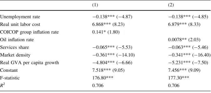
A final exercise consists of a multivariate regression analysis aimed at determining the factors responsible for Spanish inflation. In our view, given the characteristics of the Spanish economy, all the signs from the multivariate analysis are plausible, in terms of the Phillips curve, the non-wage price pressure, the disinflationary competition and sectoral specialization patterns—given the problems and rigidities of the goods and labor markets in Spain. Finally, the negative sign of the coefficient on real GVA per capita growth does not support the validity of the Balassa–Samuelson effect.

The remainder of our article is structured as follows. Section2conducts a review to further contextualize our work in the related literature. Section3 presents the PANIC approach. Section4makes a description of the inflation data employed and analyzes the choice of the break considered. Section5 comments on the results obtained from the PANIC analysis and provides an alternative test of pairwise convergence. Section6 carries out an analysis utilizing some additional variables other than inflation, also paying attention to CPI weightings and testing the Balassa– Samuelson hypothesis. Finally, Sect.7concludes.

6

Galı´ and Lo´pez-Salido (2001), within the framework of the recent literature about the Phillips curve— see Galı´ and Gertler (1999)—, emphasize the role of wage frictions and the backward-looking component of inflation expectations. That second factor is also stressed by Fabiani et al. (2006). Restoy et al. (2005) point to the problem of the Spanish dual inflation. Likewise, they highlight the relevant role of wage indexation. Caraballo and Dabu´s (2013) and Caraballo and Usabiaga (2009a,b) present evidence for the presence of menu costs—or other nominal rigidities—in the determination of Spanish consumer and producer prices. The latter also focuses on the vulnerability of Spanish inflation to adverse oil shocks. Finally, we should underline that the labor reforms undertaken between 2010 and 2012 (Bentolila et al.

2 Literature review

2.1 Disinflation and inflation convergence: evidence and lessons for Latin America

One geographic area that has long struggled to end high and chronic inflation is Latin America. Latin American countries have endured bouts of high inflation and hyperinflation in the recent past and some of them (mainly Venezuela and Argentina) are currently grappling with this scourge again. For the remaining countries, on a general basis inflation has come down from high numbers in the 70s, 80s and 90s to more moderate rates in the present decade. It is worth mentioning that, in addition to opening themselves up to trade, countries like Mexico, Chile, Peru, Colombia and Uruguay are known to have been quite successful in bringing to birth a full-fledged inflation-targeting regime.7 The inflation rates after the implementation of the new framework plummeted in all these economies.8 Additionally, to be sustainable, this monetary arrangement calls for the conduct of a more rigorous fiscal policy which may have also played some role in helping drive inflation down over time.9It is important to mention that the evidence mostly points to the existence of a positive relation between the interplay of globalization and monetary policy, via the incentives that the former raises for central banks to behave prudently, and disinflation.

To our knowledge, the literature on the effects of the interaction of the aforementioned factors on inflation convergence within countries is fairly scant, especially in Latin America. Intuitively, a country’s regions, subject to the same monetary policy and roughly similar structural reforms and fiscal policies, should in principle experience long-run inflation convergence (Yilmazkuday 2013). More-over, if, as a consequence of a further step taken toward a deeper economic and monetary integration, some of these joint policies are carried out at a supranational level, while others are influenced or restricted by common rules set at the same level, a stronger sub-national inflation convergence is likely to occur, at least throughout the initial stages of the process.

From a policy-oriented perspective, we view this analysis as relevant since non-negligible differences in real interest rates could arise within the country did regional inflation rates differ from each other, due for instance to distinct cyclical positions across these regions’ economies, thereby perpetuating diverging economic performances at regional level. Besides, persistent differences in inflation might reflect permanent structural rigidities that prevent the regions hardest hit by shocks from adjusting swiftly.

7

Brazil is another inflation targeter in the region, but we have elected to leave it out of our comments as it is a relatively closed economy.

8 _{See Blake et al. (2015), for an application to Chile, Colombia, Mexico and Peru, and Garcı´a-Solanes}

and Torrejo´n-Flores (2012), for the same countries plus Brazil.

9 _{To get a sense of how important fiscal discipline can be under an inflation-targeting regime, see}

Let us now pick two countries, Mexico and Peru, among the ‘‘globalizers’’ we just chose because of data and empirical evidence availability. In the case of the former, to the best of our knowledge, only studies on regional (relative) price convergence can be found. Sonora (2005) tests whether the PPP hypothesis holds across Mexico’s main cities. His results show that there is relative price convergence in the long run. Furthermore, he also suggests that prices are relatively flexible, which runs counter to the slower long-run price convergence found for US and Canadian data. Go´mez-Aguirre and Rodrı´guez-Cha´vez (2013a,b) also examine price convergence across the main Mexican cities by employing panel data unit root tests. Their findings in both papers coincide with Sonora’s: absolute price parity holds in the long run. As far as inflation convergence is concerned, a quick inspection of Mexican provincial inflation rate data (Instituto Nacional de Estadı´stica y Geografı´a) provides a clue as to whether there has been regional/ provincial inflation convergence over time. A simple sigma-convergence analysis leads us to think this has been the case. Mexico is a NAFTA member and is therefore relatively integrated by commercial and financial ties with the US and Canada, and with the rest of the world as well. This relevant economic integration, coupled with sound economic policies, in part due to the necessary consistency with the status of being a more open economy, may have contributed to this regional/ local inflation convergence coming about over time.

On the Peruvian economy, Winkelried and Gutie´rrez (2012) show that the central bank of Peru, by having targeted Lima’s inflation, has been in fact influencing the economy-wide inflation,10which in the end constitutes an indication that regional inflation rates have converged over time. By means of a multivariate dynamic model of inflation comprising the main nine regions in the country, they conclude that the relative PPP holds among pairs of regional inflations. Again, Peru is an economy whose recent progress on the macroeconomic and institutional front has been remarkable. This virtuous cycle, in a way sparked by these aforementioned good policies,11 has materialized itself in considerable economic growth rates and low inflation.12A steady convergence in regional inflation is an expected outcome given the policies put in place from the 90s onwards.

As may be seen, the Spanish case that we choose to analyze in this article can be generalized to other open economies, such as several in Latin America, to the extent that these latter economies share certain characteristics with the Spanish economy (degree of openness, central bank behavior, fiscal policy stance, etc.).

10

As the authors themselves say, Peru is a heavily centralized country, as Lima concentrates about a third of the country’s population and used to represent more than 70 % of national expenditure.

11_{Some economists assert that ‘‘good luck’’ seems to have played a greater role than good policies have}

in causing Peru’s notable economic performance—see for example Mendoza (2013).

12_{Although risks stemming from external shocks like the fall in commodity prices on international}

2.2 Disinflation and inflation convergence within a European context

After the view of the processes of disinflation and convergence in inflation in Latin America, we are going to concentrate now on the Spanish case, logically placed within the euro area context. The process of Spanish disinflation in the past decades is well-known, and it has been widely studied using mainly the SVAR method-ology—see the survey by Go´mez and Usabiaga (2001).

As regards convergence, there exist several strands in the literature covering price level convergence, inflation convergence and inflation differentials. Although logically those literatures are closely related, each one of those research lines has some economic and econometric specific features. On the inflation rates and their convergence, main topic of our paper, there are more country-based case studies than region-based ones. For instance, there is a lot of literature on this topic for Western European countries. One can also find abundant literature on the euro area countries’ inflation differentials—see de Haan (2010) for a survey as well as several ECB publications.

Although with slight caveats, related to the price indices, the time periods, or the countries considered, in general, for the euro area countries inflation convergence has been reported—see for instance Montuenga-Go´mez (2002), Busetti et al. (2007) and Beck et al. (2009)—, mainly before the mid-90s. However, there still exist significant and persistent inflation differentials in the euro area (de Haan 2010), which even allow classifying countries under different categories or clusters—see for instance Montuenga-Go´mez (2002) and Busetti et al. (2007).

Beck et al. (2009, p. 153), with the euro zone in mind, present the following classification of the potential underlying factors in inflation differentials—de Haan (2010) uses a roughly similar classification—: (1) differences between the actual positions of the economies within their business cycles, asymmetric shocks, and asymmetric effects of area-wide impulses such as monetary impulses, exchange rate movements or oil price changes. (2) The Balassa–Samuelson effect. (3) Inappro-priate domestic policies or other unwarranted domestic developments such as misaligned fiscal policies, immoderate wage evolution, or other production input factor price developments. (4) Nominal wage and price rigidities. Beck et al. (2009) point out that the most worrisome factors are those of the two last types.

observed long-run differences are chiefly caused by inefficiencies in factor markets and region-specific structural characteristics. They also remark that there is considerable heterogeneity in the economic structure of euro area regions such that even symmetric impulses—such as a monetary policy shock—can have heteroge-neous effects.

From the analysis of the regional inflation rates of the euro area countries, Beck et al. (2009) state that national factors matter. Thus, the dispersion is higher among the regions of all the European countries analyzed (Austria, Finland, Germany, Italy, Norway and Spain) than among the regions of each country. In addition, differences are substantially more pronounced across regions than across country averages. These authors assert that the strong influence of the national factor very likely stems both from nationally conducted fiscal policy and nationally determined labor market institutions. In comparison to US regional inflation rates, the euro area regional rates show a slightly higher degree of dispersion and persistence. Using a factor model, Beck et al. (2009) find that the variation in euro area regional inflation rates is explained following these proportions: area-wide factors 50 %, national factors 32 %, regional elements 18 % (Spain: national factors 26.8 %, regional factors 24.6 %). They come to the conclusion that the Spanish differential in this respect can probably be explained by the relatively high degree of independence that Spanish regions enjoy.

Several works highlight that the monetary policy followed by EMU could have generated convergence effects also at regional level, due to its effect on expectations and other factors. For instance, Beck et al. (2009) state that the area-wide monetary policy can considerably contribute to regional inflation stabilization even though it cannot take regional developments into account when making its decisions. Apart from Beck et al. (2009), other works also report regional inflation convergence. For instance, Busetti et al. (2006) conduct an analysis of the price level and the inflation rate for the monthly series of the CPI in 19 Italian regional capitals over the 1970–2003 period, concluding that the convergence process is stronger for the inflation rate. Gozgor (2013) also observes convergence in Turkish regional inflation rates (period 2004–2011).

Finally, in the present study we can state that when we disaggregate provincial CPI-based inflation rates into province-level inflation rates of the 12 COICOP groups of goods and services over the 1994–2015 period, we are able to uncover some interesting patterns. With the exception of the Communications group involving mainly non-tradables, all the other groups of goods and services appear to exhibit a high degree of convergence among pairs of inflation rates across provinces. This indicates that convergence in provincial inflation rates is widespread across groups of goods and services, irrespective of the tradables/non-tradables distinction.

It is well accepted that the Balassa–Samuelson effect fails to account for the euro area inflation dynamics—see ECB (2005), Rogers (2007) and Beck et al. (2009). The Spanish economy is not an exception in this regard, maybe because some of its assumptions do not hold in that economy; for instance features like a rather centralized wage determination, a low labor mobility, etc. (Jimeno and Bentolila

1998), run counter to its central assumptions. Juselius and Ordo´n˜ez (2009) point out that the potential Balassa–Samuelson effect has more influence over the high unemployment than over prices. Rabanal (2009) concludes that the Balassa– Samuelson effect does not appear to be an important driver of the inflation differential Spain-EMU during the EMU period, although a gap in labor productivity between tradable and non-tradable sectors can be noted. In addition, Alberola and Marque´s (2001) reject the Balassa–Samuelson hypothesis at Spanish regional level. Finally, in Beck et al. (2009) this theory is not supported for the Spanish regions. To sum up, there is overwhelming evidence against the relevance and explanatory power of that hypothesis for the Spanish economy. Our results do not support the Balassa–Samuelson hypothesis since there is not a significantly higher degree of convergence among pairs of provincial inflation rates for tradables, relative to non-tradables (of course bearing in mind the exception of the Communications sector). Likewise, our multivariate regression analysis provides evidence of a significantly negative impact of real GVA per capita growth on the inflation rate, which runs counter to the positive effect that would be predicted according to the Balassa–Samuelson hypothesis.

3 PANIC approach

Different from most second-generation panel unit root tests that only allow for weak forms of cross-sectional dependence (contemporaneous short-run cross-correlation), some panel unit root tests relying on linear factor models can enable stronger forms of cross-dependence such as cross-sectional cointegration. Among the panel procedures that use a factor structure are Moon and Perron (2004), Pesaran (2007b) and Bai and Ng (2004a, b, 2010). While Pesaran (2007b) just allows for one common factor, Moon and Perron (2004) and Bai and Ng (2004a,b,2010) allow for multiple common factors. Nevertheless, only the panel tests of Bai and Ng (2004a,

observed series and the common factor would be cointegrated. In that particular case of cross-cointegration, the tests of Pesaran (2007b) and Moon and Perron (2004) probably display size distortions, as the common trends may be confused with the common factors and thus taken away from the data in the defactoring process. Hence, the tests on the observed series seem to yield stationarity if the remaining idiosyncratic component is stationary, in spite of the presence of non-stationary common factors.

Let us model the observed data on inflation rates (denoted bypit) as the sum of a

deterministic part, a common component and an idiosyncratic error term:

pit¼Ditþk0iFtþeit ð1Þ

whereki is an r1 vector of factor loadings, Ft is an r1 vector of common

factors, and eit is the idiosyncratic component. Dit can contain a constant and a linear trend. SincekiandFt can only be estimated consistently wheneitIð0Þ, we

estimate a model in first-differences like Dpit¼k0iftþzit, where zit¼Deit and ft¼DFt.13We next use principal components to estimate the common factors (^ft),

the corresponding factor loadings (k^i) and the residuals (^zit¼Dpitk^0i^ft), so that we

preserve the order of integration ofFt andeit. As in Bai and Ng (2002), we nor-malizepitfor each cross-section unit to have a unit variance. The common factors

and the residuals are then obtained as follows: Ft^ ¼Pts¼2f^s and ^eit¼

Pt s¼2zis^ ,

which can be used to test for a unit root in the common and idiosyncratic com-ponents, respectively.

3.1 Determining the number of common factors

Prior to testing for a unit root in the common and idiosyncratic components, we make use of information criteria to set the number of common factors contained in the panels of inflation rate series. We do so with the BIC3information criterion:

BIC3ðkÞ ¼r^2eðkÞ þkr^ 2 eðkmaxÞ

ðNþTkÞlnðNTÞ

NT

ð2Þ

wherekis the number of factors included in the model,r^2

eðkÞis the variance of the

estimated idiosyncratic components, and r^2

eðkmaxÞ is the variance of the

idiosyn-cratic components estimated with the maximum number of factors (kmax=5).14 The optimal number of common factors (k^) is chosen by applying arg min0k5BIC3ðkÞ. The BIC3is elected over other alternatives (like the ICp

information criteria) because for a general enough framework in which the idiosyncratic errors can be serially correlated and cross-correlated, the BIC3

13_{This representation amounts to the factor model with a constant. For the representation in the case of a}

specification with a trend, we refer to Bai and Ng (2004a, p. 1137).

14

criterion shows very good properties (Bai and Ng 2002). Likewise, Moon and Perron (2007) point out that the BIC3 criterion performs better in selecting the number of factors when min(N,T) is small.

3.2 Analysis of the idiosyncratic component

Before digging deeper into the methodology behind the PANIC approach, it is worth noting that the unit root tests of Bai and Ng (2004a,2010) and the stationarity tests of Bai and Ng (2004b) have been combined, always within the PANIC framework, as dictated in the original articles.15 Bai and Ng (2004a) estimate standard Augmented Dickey–Fuller (ADF) specifications for a unit root in the idiosyncratic components:

De^it¼di;0e^i;t1þ

Xpi

j¼1

di;jDe^i;tjþuit ð3Þ

The ADFt-statistic for testingdi;0 ¼0 is denoted by ADFe^cðiÞor ADFse^ðiÞfor the

cases of only a constant and a constant and a linear trend in specification (1), respectively.16 To raise statistical power, Bai and Ng (2004a) deploy pooled statistics based on the Fisher-type inverse Chi square tests of Maddala and Wu (1999) and Choi (2001). Lettingpc

^

eðiÞbe thep-value associated with ADF c

^

eðiÞ, the

pooled statistics are constructed as follows17:

Pc_e^¼ 2X

N

i¼1

logpc

^

eðiÞ ! d

x2_ð2NÞ forNfixed; T ! 1 ð4Þ

Z_ec_^¼ PN

i¼1logpce^ðiÞ N

ffiffiffiffi

N

p !d Nð0;1Þ forN; T ! 1 ð5Þ

We also employ the two Moon and Perron (2004) type pooled tests utilizing the PANIC residuals to estimate a bias-corrected pooled PANIC autoregressive estimator, and a panel version of the Sargan–Bhargava (1983) statistic using the sample moments of the residuals without the need to estimate the pooled autoregressive coefficients. A great advantage of the PANIC pooled statistics of

15_{The use of unit root statistics (for the case of testing the unit root null hypothesis) along with}

stationarity statistics (for the case of testing the stationarity null hypothesis) allows us to carry out a confirmatory analysis of the stochastic properties of the inflation rate series. See more details in Shin and Snell (2006, p. 136).

16

The asymptotic distribution of ADFce^ðiÞis the same as the Dickey–Fuller distribution for the case of no

constant, while that of ADFs

^

eðiÞis proportional to the reciprocal of a Brownian bridge. 17

The same holds for the case of a trend, whereps

^

eðiÞis thep-value associated with ADF s

^

eðiÞ. The pooled

statistics for the trend specification are denoted asPse^andZes^. Note that we do not pool individual unit root

tests for the observed series, since under a factor structure the limiting distribution of the test would contain terms that are common across units. However, ‘‘pooling of tests fore^itis asymptotically valid

Bai and Ng (2010) is that there is no need for least squares linear detrending that could give rise to a fall in statistical power.

3.3 Analysis of the common component

An ADF test is used to test for non-stationarity in the common factor. When the panel only has one common factor, as it is our case, we estimate an ADF specification for bFt with the same deterministic components as in model (1):

DFt^ ¼Dtþc0Ft^1þ

Xp

j¼1

cjDFt^jþvt ð6Þ

The corresponding ADFt-statistics are denoted by ADFc_F^and ADFs_F^and follow the limiting distribution of the Dickey and Fuller (1979) test for the specifications with only a constant, and a constant and a trend, respectively.

3.4 Stationarity tests for the common and idiosyncratic components

As noted above, the stationarity test of Kwiatkowski et al. (1992, KPSS) is used and applied to both the common and idiosyncratic components following Bai and Ng (2004b). The univariate KPSS tests for the idiosyncratic components are denoted by

Sc_e^ðiÞandSs_e^

0ðiÞdepending on whether trends appear or not in the specification, and

the tests for the common factors areSc_F^andSs_F^. The limiting distribution ofSc_F^and

Ss ^

Fare those derived by KPSS for the cases of a constant, and a constant and a linear

trend, respectively. However, the limiting distribution for testing eit^ depends on whether Ft^ is I(0) or I(1). If all factors are I(0), Sc

^

e0ðiÞ and S s ^

e0ðiÞ follow the

distribution of the KPSS tests for the cases of a constant, and a constant and a trend, respectively. But if the factor isI(1), as it is our case, stationarity in the idiosyncratic component implies cointegration between the observed series and theI(1) common factor. In that case, we have to employ univariate cointegration tests denoted by

Sc

^

e1ðiÞ andS s ^

e1ðiÞ, which have the limiting distribution of the cointegration test of

Shin (1994).

With respect to the computation of pooled statistics, when the common factors are stationary, the p-values associated with the univariate KPSS tests for the idiosyncratic components can be used to compute the pooled tests of Maddala and Wu (1999) and Choi (2001). Otherwise, pooling is not valid since the non-stationarity of the common factors is transmitted to the residuals under the null hypothesis of stationarity because it does not fade away even asymptotically.18

4 Inflation data and the timing of the break

4.1 Data description

The main data we deploy in this article are CPI data,19spanning from 1955.1 until 2014.4 at a monthly frequency, and they are sourced from INE (Instituto Nacional de Estadı´stica). We avail ourselves of year-on-year numbers so as to avoid the seasonality problem. The data correspond to provincial capitals (up to 1992) and to provinces themselves thereafter. Connecting both kinds of series, without manip-ulating them, proves unproblematic. We have only engaged in two very specific manipulations of our inflation series in order to correct for two anomalous figures related to the province of Zamora, in 1960.1 and 1961.1.20In spite of having access to previous years, we have decided to stick to 1955 as the first year of our study mainly for three reasons: (1) because we would not like to go too far back in time, since our analysis neither aims to adopt an economic history approach nor to deal with episodes too far back in history. (2) Because data might cease to be statistically trustworthy as we move backwards in time, this trust being a fundamental factor for the econometric analysis conducted. (3) Because for additional assessments we make use of some other series, in addition to inflation, which mostly start after 1955.

Our work’s basic data (inflation rate) is a panel made up of 50 (N, provinces) by 712 (T, months). Nevertheless, for our purposes, the aforesaid panel is split into two different sub-samples. Indeed, in what follows, our article attempts to clarify whether the behavior of the provincial inflation rate varies between sub-periods. But before turning to the PANIC analysis, we next try to determine through econometric techniques where the break is located, as a better alternative to exogenously imposing it.

4.2 Determination of the endogenous break in inflation

In order to determine the most likely break in the provincial inflation rate series, we need to find the most likely common structural shift that is affecting all the series simultaneously.21The avenue we take for that is to test for structural instability in the common stochastic trend that is driving all province-specific inflation rate series over the whole period. To identify the break location we follow the procedure proposed by Lee and Strazicich (2003). Unlike the Lumsdaine and Papell (1997) unit root test which is derived assuming no breaks under the null hypothesis, the unit root test of LS allows for breaks under both the null and alternative hypotheses. As pointed out by LS, rejection of the null with the Lumsdaine and Papell (1997) test only indicates rejection of a unit root without breaks, whereas the alternative does

19

Unfortunately, the existing data do not enable us to conduct an analysis of production prices akin to the one implemented in this work.

20

Given that they were a very low value and a very high one, respectively, we have opted to give it the second lowest value and the second highest value, respectively, as they were more suitable altogether.

21

not necessarily imply stationarity around a shifting trend. Using the Lagrange Multiplier (LM) score principle, LS estimate the following regression:

Dpt¼d0DZtþ/St~1þ

Xk

1

ciDSt~iþet ð7Þ

whereSt~1 represents the detrended series such thatSt~ ¼ptw~XZtd~, fort=2 …T.d~is a vector of coefficients estimated from the regression ofDptonDZt and

~

wX¼p1Z1d~, wherep1andZ1 are the first observations ofptandZtrespectively,

andZtis a vector of exogenous variables defined by the data generation process of the inflation rate series. The crash model allows for one shift in the intercept such thatZt¼½1;t;DU1t0.22The mixed change model allows for one change in level and

slope, as given byZt¼½1;t;DU1t;DT1t0.

The unit root null hypothesis is given by/¼0 versus the alternative that/\0, and the LM t-statistic is defined by ~s(t-statistic testing the null hypothesis that

/¼0). The minimum LM unit root t-statistic determines the endogenous location of the break (k¼TB=T) by using a grid search over all possible break points such

that LMs¼infks~ðkÞ. To correct for serial correlation, we control for a sufficiently

large number of augmentation terms (k) by employing the general to specific approach proposed by Ng and Perron (1995), settingkmax=12.23

For the crash model the mean shift is located at July 1978, whereas for the mixed change model the shift in mean and slope appears located at April 1979. Given the non-trending behavior exhibited by the inflation rate, we base our conclusions on the crash model which points to the existence of a mean shift at July 1978. The cross-province mean inflation rate for the first regime equals 9.4 %, whereas it equals 5.8 % for the post-break regime, implying a clear downward shift in the mean inflation rate after the break took place. In addition, it is interesting to point out that the value of the LM unit root test of LS for the crash and mixed change models is -2.155 and -2.795, respectively, both values well below (in absolute terms) the respective 10 % critical values (-3.504 and-4.989). This indicates the existence of a unit root in the common factor for the whole period after accounting for one structural break in the mean (and slope) of the series.

For robustness purposes, we also applied the generalized least squares (GLS)-based unit root tests allowing for one break under both the null and alternative hypotheses proposed by Carrio´n-i-Silvestre et al. (2009). These tests include the class of modified tests (M tests), originally proposed by Stock (1999), and later extended by Perron and Ng (1996) and Ng and Perron (2001). The latter apply

local-22

Our model allows for a structural break under the null and the alternative, thus controlling for a change in level under the alternative and for a one-period jump under the null hypothesis.

23_{To sum up, this approach presents several methodological advantages. First, the distribution of thet}

to-unity GLS detrending instead of ordinary least squares (OLS) when estimating the deterministic components of an ADF regression (see Elliot et al.1996) so that important gains in statistical power can be achieved. More specifically, we employ the ADFGLS test first proposed by Elliot et al. (1996), which is the t-statistic for testing the existence of a unit root with a specification where the underlying series is detrended with GLS prior to estimation by OLS. TheMGLS_{-class of tests includes}

MZGLS

a and MZGLSt which are modified versions of theZaandZtPhillips and Perron

(1988) tests, MSBGLS _{which is a modified version of the Sargan and Bhargava}

(1983) test, the feasible point optimal test ðPGLS_T Þand the modified feasible point optimal testðMPGLS

T Þ.

24_{In this case, the break is located at August 1977, which is}

very close to the break date identified with the LS procedure. Since a visual inspection of Fig.1appears to favor a major downward shift in mean inflation in the middle of 1978, we stick to the result obtained from the application of LS methods. Still, it is reassuring that both methods render fairly similar results. Not surprisingly either, none of the GLS-based unit root tests is able to reject the unit root null hypothesis at conventional significance levels,25thus supporting the non-stationarity of the common factor.

Our initial working hypothesis, which turns out to be confirmed throughout our analyses, is that from the break identified (1978.7) up to the present day a number of relevant economic, political and institutional changes, both at the national and international levels, have necessarily left their imprints on the inflation rate, among other variables. This changing pattern is intended to be captured, in a first step, via PANIC, and in a second step, via other convergence assessments.

The break identified can be largely thought of as a turning point in Spanish economic policy relative to Franco’s dictatorial regime, leading to a period of a high reformist vigor brought about by the new democratic period that encompassed almost every economic area, both within the country itself and further afield, spurred by the firm intention of Spain to access to the European core. As regards Spanish internal policy, which has been progressively constrained by the European integration process, after the Pactos de la Moncloa (1977)—a battery of urgent policy measures in response to the peak in inflation—, one of the first measures taken was the adoption of the medium-term economic program 1983–1986 (updated twice afterwards). In this program, on the one hand, some adjustment policies were put into place with the aim of correcting the main macroeconomic imbalances, and, on the other hand, several structural reforms were fostered in order to better articulate the productive fabric of the country and enhance the efficient functioning

24

For these tests to exhibit good size properties, it is crucial to select the appropriate lag truncation (k) of the ADF specification. For that purpose, Ng and Perron (2001) develop the modified Akaike information criterion which aims at selecting a relatively long lag-length in the presence of a large negative moving average root (thus preventing size distortions) and a short lag-length when that root is not present (thus avoiding unnecessary loss of power). In our application, we take a maximum lag truncation of 12. This analysis is conducted with GAUSS routines kindly provided by Pierre Perron athttp://people.bu.edu/ perron/code/Replication-codes-ET-2009.zip.

25

of the markets.26It is also indisputable that the initiatives in favor of the European integration, and the legislative alignment that ensued from that, were crucial during those years which ended with Spain entering the European Economic Community (EEC) on January the 1st 1986. Within this process, the Maastricht Treaty called for central banks’ independence of those countries aiming to join the Single Currency, which in the case of Spain led to the approval of the Law of Autonomy of the Bank of Spain (Law 13/1994). In the context of EMU, an inter-annual inflation target around 2 % was established.27

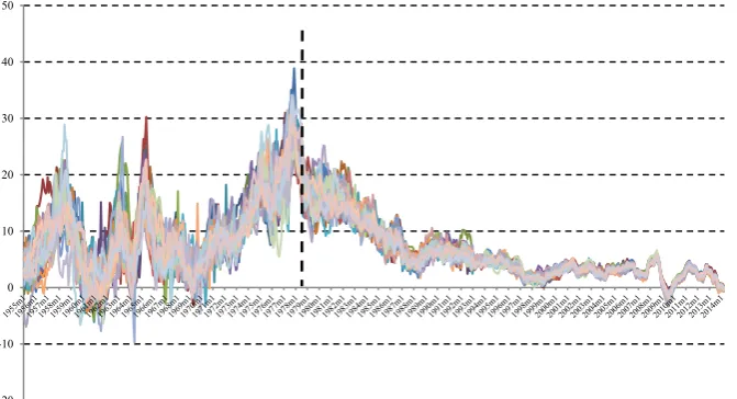
In case the justification of the timing of the break, based on institutional, political and economic grounds, was deemed insufficient, Fig.1 plots the evolution of the provincial inflation rates for both periods analyzed. Even at first glance, it is easily observable that the nature of the series appears to have undergone a transformation between periods. Apart from a lower average inflation in the second period,28even in those months in which inflation is at similar levels across both periods, a lower dispersion for the second one is perceived.

-20 -10 0 10 20 30 40 50

Fig. 1 Evolution of Spanish provincial inflation rates. Inter-annual data. 1955.1–2014.4

26_{On the adjustment measures, in addition to a strong commitment to income policies, great importance}

was placed on a restrictive monetary policy stance and on fighting inflation. This economic strategy was generally perceived to be the appropriate one at that time, following the second oil shock. As for the structural reform package, during those years a multitude of measures were conducted, like the industrial and energy restructuring, transformation of public enterprises, etc. We should also remember that the Spanish labor market approached the way a genuine market is supposed to function essentially from the break proposed onwards, right after trade unions were legalized in 1977, and the emergence of Workers’ Statute in 1980.

27_{On the European integration process, from an economic perspective, see for example Baldwin and}

Wyplosz (2013). From a regional point of view, see for example Cuadrado-Roura and Parellada (2002), Fingleton (2003) and Maza and Villaverde (2011).

28_{It should be remembered that there exists a strand of literature on the positive relation between average}

5 Analysis of the PANIC results

5.1 Analysis of cross-sectional dependence

Before we implement the PANIC analysis, two cross-dependence tests are applied to ascertain the likely existence of cross-correlation in inflation innovations for the two panels of inflation rate series under scrutiny. These tests are those put forward by Breusch and Pagan (1980) and Pesaran (2004). Pesaran’s test rests on the average of pair-wise correlation coefficients (q^ij) of OLS residuals derived from standard

ADF regressions for each individual. The order of the autoregressive model is selected using the t-sig criterion in Ng and Perron (1995), with the maximum number of lags set at p¼4ðT=100Þ1=4. This test adopts the form

CD¼pffiffiffiffiffiffiffiffiffiffiffiffiffiffiffiffiffiffiffiffiffiffiffiffiffiffiffiffiffiffiffi2T=ðNðN1ÞÞ P_iN_¼11PN_j¼iþ1q^ij

!d Nð0;1Þ. The CD statistic tests the

null hypothesis of cross-sectional independence, is distributed as a two-tailed standard normal distribution and exhibits good finite-sample properties. Moreover, Breusch and Pagan (1980) test the null hypothesis of cross-sectionally independent errors via the following LM statistic: CDlm¼TPNi¼11

PN j¼iþ1q^

2

ij!

d

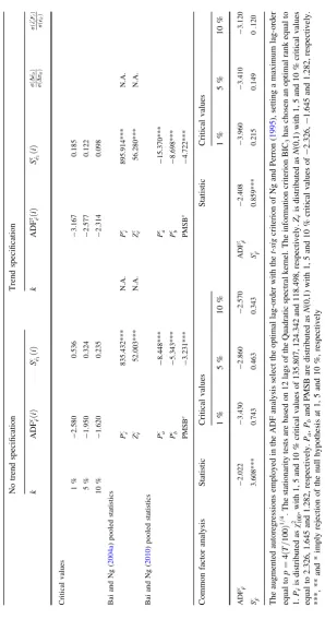
x2_NðN1Þ=2Þ. Even though throughout the analysis all the outcomes for the specification both with and without trends are computed, as inflation is often portrayed as a variable of the second type, we concentrate on the evidence obtained for the specification with no trends.29 For the two panels we are able to reject the null hypothesis of cross-sectionally independent errors at the 1 % level of significance with both the CD test and the Breusch and Pagan LM test (Table1). This in turn supports the use of PANIC that allows for cross-sectional dependence so that large size distortions in the tests are avoided—see O’Connell (1998), Maddala and Wu (1999) and Banerjee et al. (2005).

5.1.1 Optimal number of common factors

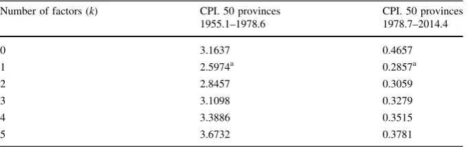
Before testing for a unit root in the idiosyncratic series and common factors in which the inflation rate series forming the two panels are broken down, the common factors are estimated through principal components and the number of factors present in the two panels investigated is then selected. Table2displays the results from the application of the BIC3criterion to the two panels of inflation series. This criterion picks one common factor for the two panels. Since Bai and Ng (2002) provided evidence that the BIC3 criterion performed remarkably well in the presence of cross-correlations and Gengenbach et al. (2010, p. 134) offered simulation evidence of the superior performance of the BIC3 criterion for

short-Npanels, and given the difficulty in establishing the number of common factors in panels with relatively shortN, we will undertake the decomposition of the inflation rate series as if there existed one common factor, as specified by the BIC3criterion.

29_{As will become apparent below, the main results are fairly robust to the inclusion of a linear trend in}

5.2 PANIC analysis of the panel of CPI-based inflation rates for the Spanish provinces

5.2.1 First period results

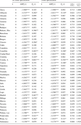
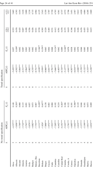
Table3 presents the results of the univariate ADF and KPSS tests applied to the idiosyncratic series, the respective univariate tests for the common factor as well as the pooled statistics of Bai and Ng (2004a, 2010) for the panel of CPI-based inflation rate series for the 50 Spanish provinces over the period 1955.1–1978.6. The aim is to determine the source of non-stationarity in Spanish provincial inflation, i.e., whether the common and/or idiosyncratic series are non-stationary. In this case, the BIC3procedure selected only one common factor.

Furthermore, as the univariate statistics applied to the common factor yield unclear evidence as to whether the common component is stationary or not (since the ADFc_F^and ADFs_F^ statistics favor the stationarity hypothesis, whilst the KPSSc

^

F and KPSS

s ^

F

statistics lend support to the unit root hypothesis), we apply the IPC1, IPC2and IPC3 information criteria of Bai (2004) as an alternative and more reliable methodology to determine the number of non-stationary common factors in the panel (setting the

Table 1 Cross-sectional dependence analysis

No trend specification Trend specification CPI. 50 provinces

1955.1–1978.6

CPI. 50 provinces 1978.7–2014.4

CPI. 50 provinces 1955.1–1978.6

CPI. 50 provinces 1978.7–2014.4 LM test 491.383a 2383.475a 488.076a 2390.468a

CD test 152.845a 338.290a 152.327a 338.767a

The CD-statistic and the LM-statistic test for the null of cross-sectional independence. The CD-statistic is distributed as a two-tailed standard normal distribution and the LM-statistic as av2

NðN1Þ=2distribution a

Implies rejection of the null hypothesis at the 1 % significance level

Table 2 BIC3(k) information criterion

Number of factors (k) CPI. 50 provinces 1955.1–1978.6

CPI. 50 provinces 1978.7–2014.4

0 3.1637 0.4657

1 2.5974a 0.2857a

2 2.8457 0.3059

3 3.1098 0.3279

4 3.3886 0.3515

5 3.6732 0.3781

a

Table 3 PANIC analysis of CPI inflation. Spanish provinces. 1955.1–1978.6 No trend specification Trend specification

k ADFc

^

eðiÞ S

c

^

e1ðiÞ k ADF

s

^

eðiÞ Sse^1ðiÞ

rðDe^itÞ

rðDpitÞ

rðk0

iFtÞ

rðe^itÞ

Table 3 continued

No trend specification Trend specification

k ADFc

^

eðiÞ S

c

^

e1ðiÞ k ADF

s

^

eðiÞ Sse^1ðiÞ

rðDe^itÞ

rðDpitÞ

rðk0

iFtÞ

rðe^itÞ

Santa Cruz de Tenerife

2 -3.187*** 0.475** 2 -4.164*** 0.057 0.947 0.607

Segovia 0 -4.200*** 0.069 0 -4.299*** 0.052 0.641 3.076 Sevilla 0 -4.951*** 0.182 0 -4.991*** 0.066 0.632 2.607 Soria 3 -2.820*** 0.115 3 -2.792** 0.105* 0.725 2.173 Tarragona 3 -4.006*** 0.097 0 -4.002*** 0.096 0.645 3.100 Teruel 1 -3.876*** 0.199 1 -4.062*** 0.147** 0.778 2.225 Toledo 4 -3.443*** 0.704*** 4 -3.980*** 0.062 0.816 1.779 Valencia 0 -5.692*** 0.096 0 -5.747*** 0.049 0.687 1.853 Valladolid 0 -3.199*** 0.107 0 -3.241*** 0.081 0.744 1.807 Zamora 0 -2.091** 0.139 0 -2.738** 0.129** 0.751 1.290 Zaragoza 1 -5.986*** 0.036 1 -6.000*** 0.035 0.581 3.021 Critical

values

1 % -2.580 0.536 -3.167 0.185

5 % -1.950 0.324 -2.577 0.122

10 % -1.620 0.235 -2.314 0.098

Bai and Ng (2004a) pooled statistics

Pc

^

e 809.457*** N.A. Pse^ 810.675*** N.A.

Zc

^

e 50.166*** N.A. Zes^ 50.252*** N.A.

Bai and Ng (2010) pooled statistics

Pc

a -70.372*** Psa -51.347*** Pc

b -17.300*** Psb -18.592***

PMSBc _{-4.972*** PMSB}s _-6.358***

Common factor analysis

Statistic Critical values Statistic Critical values

1 % 5 % 10 % 1 % 5 % 10 %

ADFc

^

F -2.783* -3.430 -2.860 -2.570 ADF s

^

F -3.427** -3.960 -3.410 -3.120 Sc

^

F 1.185*** 0.743 0.463 0.343 S s

^

F 0.371*** 0.215 0.149 0.120

The augmented autoregressions employed in the ADF analysis select the optimal lag-order with thet-sig

criterion of Ng and Perron (1995), setting a maximum lag-order equal top¼4ðT=100Þ1=4_{. The}

sta-tionarity tests are based on 12 lags of the Quadratic spectral kernel. The information criterionBIC3has

chosen an optimal rank equal to 1.Pe^is distributed asv2100, with 1, 5 and 10 % critical values of 135.807,

124.342 and 118.498, respectively.Ze^is distributed asN(0,1) with 1, 5 and 10 % critical values equal to

2.326, 1.645 and 1.282, respectively.Pa,Pband PMSB are distributed asN(0,1) with 1, 5 and 10 %

maximum number of factors to five). These criteria clearly point to the existence of only one common stochastic factor.30Thus, if the common factor is found to be non-stationary, and the idiosyncratic components are I(0) stationary, there would be evidence of pair-wise cointegration among the inflation rate series pertaining to the panel.

We next turn to testing for a unit root in the idiosyncratic series. The evidence seems to mostly favor stationarity of the idiosyncratic series even at the univariate level since the unit root null is rejected with the ADF statistic for all the provincial series at the 1 % level, except for three provinces (Co´rdoba, Las Palmas and Zamora) for which the null is rejected at the 5 %. The application of the Shin statistic (as the presence of one non-stationary common factor kept us from using the KPSS test) renders confirmatory evidence of stationarity for 37 provinces. For the rest (13 provinces), the evidence appears inconclusive as the stationarity null is also rejected in this case (for 3 provinces at the 1 % level of significance, 5 at the 5 % and 5 at the 10 %), as occurred with the unit root null with the ADF statistic.31To supply evidence of the stochastic properties of the idiosyncratic component for the panel as a whole, we apply the pooled Fisher-type inverse Chi square tests of Maddala and Wu (1999) and Choi (2001) along with the PANIC pooled Moon–Perron and Sargan–Bhargava statistics. It is worth highlighting that we are able to reject the joint non-stationarity null hypothesis with the five pooled statistics at the 1 % level of significance, regardless of the inclusion of deterministic trends in the idiosyncratic series specifications. Hence, there is overwhelming evidence of the joint stationarity of the idiosyncratic component of the panel under study.

Columns 8 and 9 of Table3 show the ratio of the standard deviation of the idiosyncratic component to the standard deviation of the observed data (both expressed in first-differences), and the ratio of the standard deviation of the common component to the standard deviation of the idiosyncratic component respectively, to get a sense of the relative importance of the common and idiosyncratic components. The average values of those ratios are 0.69 and 2.32, respectively.32

Overall, the finding that the source of non-stationarity in the panel is a common stochastic trend driving the non-stationarity in the observed series has become apparent. Both this fact and the presence of a jointly stationary idiosyncratic component combine to render evidence of pairwise cointegration among the Spanish provincial inflation rate series.

5.2.2 Second period results

Table4 presents the results of the univariate ADF and KPSS tests applied to the idiosyncratic series, the respective univariate tests for the common factor as well as

30_{Unlike the information criteria to determine the optimal number of common factors (stationary and}

non-stationary) in Bai and Ng (2004a,b) that are applied to data in first-differences, the IPCp panel

information criteria to determine the number of non-stationary common factors proposed by Bai (2004) are applied to level data. In addition, the consistency of Bai (2004)’s information criteria requires the idiosyncratic component to beI(0), which we will find below to be the case.

31

These results are very similar for the trend specification.

32_{As laid out by Bai and Ng (2004b), if all variations are idiosyncratic, the first ratio should take a value}

Tabl e 4 PANI C an alysis of CPI inflation . Span ish Prov inces. 1978 .7–2014. 4 No trend specific ation Trend specific ation k ADF

cði^e

Þ

S

cð^e1

i

Þ

k

ADF

sði^e

Þ

S

sð^e1

i Þ r ð D ^eit Þ r ð D pit Þ r ð k

0Fi

t

Þ

r

ð

^eÞit

Tabl e 4 cont inue d No trend spec ification Trend specifi cation k AD F

cði^e

Þ

S

cð^e1

i

Þ

k

ADF

sði^e

Þ

S

sð^e1

i Þ r ð D ^eit Þ r ð D pit Þ r ð k

0Fi

t

Þ

r

ð

^eÞit

Tabl e 4 cont inued No trend spec ification Trend specifi cation k AD F

cði^e

Þ

S

cð^e1

i

Þ

k

ADF

sði^e

Þ

S

sð^e1

i Þ r ð D ^eit Þ r ð D pit Þ r ð k

0Fi

t Þ r ð ^eit Þ Critical values 1% -2.580 0.536 -3.167 0.185 5% -1.950 0.324 -2.577 0.122 10 % -1.620 0.235 -2.314 0.098 Bai and Ng ( 2004a ) pooled statistics P

c ^e

835.432***

N.A.

P

s ^e

895.914***

N.A.

Z

c ^e

52.003***

N.A.

Z

s ^e

56.280*** N.A. Bai and Ng ( 2010 ) pooled statistics P c a -8.448*** P s a -15.370*** P c b -5.343*** P s b -8.698*** PMSB c -3.231*** PMSB s -4.722*** Common fact or analy sis Stati stic Criti cal value s Statistic Critic al va lues 1 % 5 % 1 0 % 1 %5 %1 0 % ADF

c ^F

-2.022 -3.430 -2.860 -2.570 ADF

s ^F

-2.408 -3.960 -3.410 -3.120 S

c ^F

3.608***

0.743

0.463

0.343

S

s ^F

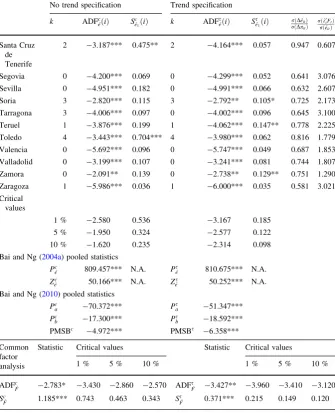
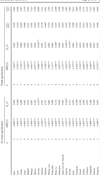
the pooled statistics of Bai and Ng (2004a,2010) for the second panel covering the period 1978.7–2014.4.

Again our aim is to discover the source of non-stationarity in Spanish provincial inflation. In this case, the BIC3procedure again selected only one common factor and there is clear evidence of a unit root in the common factor, since the unit root null is not rejected with the ADFc_F^test and the stationarity null is strongly rejected with the KPSSc_F^ statistic. This result carries over to the trend specification.

We now proceed to test for a unit root in the idiosyncratic series. The evidence appears to lend support to the stationarity of the idiosyncratic series even at the univariate level since the unit root null is rejected with the ADF statistic for 49 provinces at the 1 % significance level and for one province at the 10 % level (Bizkaia). The application of the Shin statistic yields confirmatory evidence of stationarity for 41 provinces. For the rest (nine provinces), the evidence appears inconclusive as the stationarity null is also rejected in this case (for 5 at the 5 % significance level and for 4 at the 10 %), as happened to the unit root null with the ADF statistic.33Regarding the stochastic properties of the idiosyncratic component for the panel as a whole, it should be stressed that, as in the previous case, we are able to reject the joint non-stationarity null hypothesis with the five pooled statistics at the 1 % level of significance, irrespective of the inclusion of deterministic trends in the specifications. Therefore, also for this period overwhelming evidence of the joint stationarity of the idiosyncratic component of the panel exists.

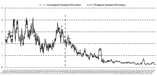
Columns 8 and 9 of Table4 supply the aforementioned ratios of standard deviations. The average values are now 0.52 and 4.22, respectively (they were 0.69 and 2.32 in the previous case). This change in those values points towards a higher importance of the common component in this second period of our analysis, which implies a stronger link among the provincial inflation rate series. This in turn indicates that convergence among provincial inflation rate series has occurred to a larger extent over the second period under study.

In sum, the panel tests applied to the idiosyncratic component support the joint stationarity of the idiosyncratic series. This, combined with the presence of a non-stationary common factor, provides evidence of pairwise cointegration among the provincial inflation rate series in both periods under scrutiny, and especially in the second one. These results fit in with prior studies about Spanish inflation persistence and the hypothesis we aim to validate in this work regarding the inflation convergence across Spanish provinces, particularly after the late 70s.34

33_{The results are very similar for the trend specification.} 34

For robustness purposes, we explicitly incorporated the possibility of structural breaks into the statistical analysis using the PANIC methodology by computing the three PANIC panel unit root tests proposed by Bai and Carrio´n-i-Silvestre (2009), which allow for multiple structural breaks and common factors. These tests include theZtest distributed as a lower-tailed standard normal distribution, the Fisher-typePmstatistic distributed as an upper-tailed standard normal distribution and the Fisher-typePstatistic

distributed as av2

2N. In computing the three panel unit root tests, we allow for five common factors as well

5.3 Pairwise test of Pesaran

As an alternative test of pairwise convergence to PANIC, we employ the pairwise test developed by Pesaran (2007a). Pairwise convergence among the N(N-1)/2 pairs (1225) of provincial inflation rates requires the existence of cointegrating relations of the series involved of the form (1,-1). This corresponds to the presence of stationarity for all possible pairs of inflation rates:dit;j¼pitp

j

t,i=1…N-1

and j=i?1…N. Following Pesaran (2007a), we test whether all cross-provincial inflation differentials (pairs) are stationary with the ADF test and a more powerful variant of the ADF statistic given by the weighted-symmetric (WS) test proposed by Park and Fuller (1995) as well as the KPSS statistic. For the former two tests, under the null of a unit root (i.e., non-convergence), the fraction of inflation rate gap pairs for which the null hypothesis is rejected should converge to the size of the unit root tests applied to individual inflation gap pairs, forN and

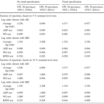
T! 1. Hence, if there is rejection of the non-convergence null for a proportion of the inflation gap pairs higher than any reasonable test size (e.g. 10 or 5 %), the evidence would be favorable to convergence. Table5 presents the results of the fraction of rejections based on the 5 and 10 % nominal level tests for both periods for the case of an intercept only and for a specification with an intercept and a linear trend. The results for the ADF and WS tests are calculated setting a maximum lag order of eight, thereby choosing the optimal lag order with either the Akaike information criterion (AIC) or the Schwarz Bayesian criterion (SBC). The results for the KPSS statistic are calculated using a bandwidth that rounds 0:75T1=3.35

As can be observed in Table5, we find evidence of a fraction of rejections close to 1 for both periods with the ADF and WS unit root tests, irrespective of the inclusion of a linear trend in the specification. This indicates that all provincial inflation rate pairs have converged to each other, thus confirming the pairwise convergence finding obtained with PANIC. However, according to the KPSS stationarity test, the null of convergence is rejected for a fraction higher than the nominal size, ranging from about 0.20 and 0.40. This would indicate the existence of a lower proportion (than 1) of inflation rate pairs converging to each other. Given the size distortions that the univariate KPSS test tends to exhibit, we base our conclusions on the basis of the ADF and WS unit root tests, which point to the existence of pairwise convergence in both periods.

6 Convergence analysis

6.1 Multivariate regression analysis

The PANIC analysis we have performed shows that, mainly in the second period, there is convergence in the provincial inflation rates. Accordingly, digging deeper into the information about convergence, in the supplementary appendix we provide