R E G U L A R A R T I C L E
Open Access
Effects of time window size and placement
on the structure of an aggregated
communication network
Gautier Krings
1*, Márton Karsai
2, Sebastian Bernhardsson
3, Vincent D Blondel
1and Jari Saramäki
2**Correspondence: [email protected]; jari.saramaki@aalto.fi 1ICTEAM Institute, Université catholique de Louvain, Avenue Georges Lemaître, 4, 1348, Louvain-la-Neuve, Belgium 2Department of Biomedical Engineering and Computational Science, Aalto University School of Science, P.O. Box 12200, FI-00076, Aalto, Finland
Full list of author information is available at the end of the article
Abstract
Complex networks are often constructed by aggregating empirical data over time, such that a link represents the existence of interactions between the endpoint nodes and the link weight represents the intensity of such interactions within the
aggregation time window. The resulting networks are then often considered static. More often than not, the aggregation time window is dictated by the availability of data, and the effects of its length on the resulting networks are rarely considered. Here, we address this question by studying the structural features of networks emerging from aggregating empirical data over different time intervals, focussing on networks derived from time-stamped, anonymized mobile telephone call records. Our results show that short aggregation intervals yield networks where strong links associated with dense clusters dominate; the seeds of such clusters or communities become already visible for intervals of around one week. The degree and weight distributions are seen to become stationary around a few days and a few weeks, respectively. An aggregation interval of around 30 days results in the stablest similar networks when consecutive windows are compared. For longer intervals, the effects of weak or random links become increasingly stronger, and the average degree of the network keeps growing even for intervals up to 180 days. The placement of the time window is also seen to affect the outcome: for short windows, different behavioural patterns play a role during weekends and weekdays, and for longer windows it is seen that networks aggregated during holiday periods are significantly different.
Introduction
Complex networks have become a standard tool for representing the interaction structure of complex systems [, ]. The strength of the network approach comes from its ability to cast the essential features of increasingly complex systems into a manageable form - in the simplest representation, interacting elements are mapped to nodes that are connected by links if they are known to interact. While this coarse-grained view has given a lot of insight into the key characteristics of such systems, it is evident that it entails several ap-proximations and underlying assumptions. The first is the criterion for the existence of links - if the interactions are not binary (on/off ) by nature, when is an interaction strong enough to be represented as a link? A common way of taking such strengths into account is to assign weights to the links of the network []. The second approximation is related
to the time domain. Standard network theory deals with networks that are either static or only slowly changing in time. However, in reality, there are typically dynamical changes in the network structure on multiple time scales. Consequently, representing an empirical system as a static network involves aggregating or integrating over the network dynam-ics over some time interval. In addition, in many cases, the interactions of the system are not continuously active. While the microdynamics of link activations may be taken into account with the temporal network framework [], for the aggregated network approach, the interaction frequencies are often used to define the edge weights. It is evident that when aggregating interactions over time, the choice of the aggregation window and its length have consequences on the characteristics of the resulting networks []. However, this issue has often been neglected in the literature; often, the aggregation interval has been dictated by the availability of data, while it would be beneficial to ensure that the network properties that one is interested in are captured by the aggregated networks.
In this paper, we address this question by monitoring and analyzing the features of net-work structure emerging from aggregation over different time intervals for an empirical data set human communication. We present a detailed study of the effects of the aggrega-tion window on the structural features human communicaaggrega-tion networks that are known to display dynamics on multiple overlapping time scales. The data comes in the form of a time-stamped sequence of mobile telephone calls between anonymized customers of a Belgian mobile operator for a period of months. This sequence is then aggregated over time to form links between customers, and key features of the resulting networks are stud-ied. Although we only study a single set of data, we expect that our conclusions generally hold for similar data sets, as the mechanisms behind network formation are expected to be rather general for such communication networks (see Discussion).
This paper is structured as follows: first, we discuss the structural and temporal inho-mogeneities that are expected to affect the features of aggregated networks. Then, we characterize the dependence of fundamental scalar measures of network structure on the aggregation interval, and address the properties of links added at different times during the aggregation procedure. We find that clustering of the network peaks at days, as the strongest links associated with dense clusters are observed early on in the process. An-other time scale is related to the stability of the aggregated networks - networks aggregated for around days display the largest similarity between consecutive windows. Moving from scalar measures to distributions, we find that the degree and weight distributions become surprisingly stationary in - weeks of aggregation time. Finally, we investigate in detail the effects of different aggregation window placements, and show that the underly-ing behavioural patterns affect the aggregated networks: on short time scales, weekends differ from weekdays, and on longer scales, holiday periods give rise to anomalies in the aggregated network structure.
Data
Our data consist of the anonymized mobile telephone call records of the customers of a Belgian mobile operator from October , to March , . Each customer is uniquely identified, and each call is associated with a time stamp and a duration. This data set has already been studied from a static perspective in several papers [, , ]. As our focus is on link dynamics, we filter out all customers who have modified their subscrip-tion plan during the data collecsubscrip-tion period. This removes new customers, and customers who have cancelled their subscription during the period. We also only concentrate on the customers of this specific operator (market share in Belgium∼%), and discard all calls to/from customers of outside operators. The above filtering yields a network that has . million customers, making over million calls during the collection period.
For reference, we also construct two randomized ensembles, based on two randomiza-tion techniques of the time stamps. For both cases, the resulting randomized reference sequences contain the same number of calls between the same individuals as the original data. In the first ensemble, the time stamps of all calls are generated uniformly at random over the complete time range, in order to remove the system-level call frequency pattern (daily and weekly pattern). In the second ensemble, the time stamps of all calls are ran-domly reshuffled, which retains the daily and weekly patterns, but removes other temporal correlations between the timings of calls of links. When aggregating over the entire obser-vation period, the call sequences from both reference models produce networks that are equal to the network from aggregating the original data. In the remaining, we will refer to these references as respectively the “uniform” and the “shuffled” references.
Network growth
Structural and temporal inhomogeneities
Figure 1 Degree, strength and weight distributions.The degree (a), strength (b) and weight (c) distributions of the aggregated network when the aggregation period covers the whole 6 months of data.
(,t); the weightwijof the link is defined as the total number of calls between iandj within the interval. The strengthsi of nodeiis then defined [] as the total number of calls whereiparticipates, and the degreekias usual as the number of links that nodeihas. As expected on the basis of earlier results [–], the probability density distributions of degree, strength, and link weights are all broad (see Figure ). Thus there is a large number of nodes that make only infrequent calls, and a large number of links that carry only a few calls. When aggregating the network over shorter time intervals, one thus expects to first discover the high-strength nodes and high-weight links that are associated with the tails of these distributions.
In the time domain, the two main inhomogeneities are related to burstiness of calls form-ing the links, and the overall circadian pattern of the system-wide call frequency. Bursti-ness of the calls is reflected in the probability distributionP(τ) of the timesτ between consecutive calls on individual edges. In Figure (a), it is seen that in line with earlier observations [, , ], the distributionP(τ) in our empirical data has a
Poissonian tail, a signature of burstiness. Such an inter-call time distribution gives rise to longer waiting times than expected if the calls were placed uniformly in time. Because of this, we expect to see slower network growth than for the uniform case. Further, as seen in Figure , the network-level call frequency clearly displays the usual daily and weekly pattern [, ], where the frequency shows two daily peaks followed by a decrease during nights. In addition, weekend activity is lower, especially for Sundays.
Evolution of network structure
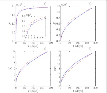
All of the above features are expected to have an effect on the properties of networks ag-gregated over growing time intervals. Let us first monitor the growth of the agag-gregated network in terms of the numbers of nodes and links and the average degree, when the networkG(t) is aggregated up to a timet. As seen in Figure (a), the number of observed nodes N(t) displays a rapid increase in the beginning of the aggregation process, such that the aggregated network contains %of the nodes aftert∼ days. This rapid in-crease is followed by slower growth as nodes with low call activity are gradually observed to make calls, joining them to the aggregated network. When compared to the uniform reference, where the time stamps of all calls are drawn uniformly at random from the entire -month interval, it is seen that the growth ofN(t) is slightly slower; however, for longer aggregation times, the difference can be considered negligible and thus the time-domain
heterogeneities have a visible effect only for short time windows. For short time windows, in addition to the slowing-down effect of burstiness, the daily pattern is seen to give rise to a stepped shape of theN(t) curve (see the inset of Figure (a)).
In contrast, the growth in the number of edgesE(t) is much more gradual, as seen in Figure (b). Here, an aggregation time of t∼ days is required for catching %of the edges of the final -month aggregated network. In addition, unlike for the number of nodes, for long aggregation times, the number of edges keeps on growing steadily and no saturation in growth is observed. This is also reflected in the growth of the average de-gree (Figure (c)). Hence, even though the number of nodes becomes fairly stable in an aggregation period of months, one cannot claim to have captured all the edges of the underlying network, and for longer windows, the average degree would still increase. This reflects the joint effect of several factors: first, as the edge weight distribution is broad, there are large numbers of edges with very low call frequencies, and observing those ev-idently takes a long time; there may be many edges where calls take place less frequently than once in six months. In addition, the ubiquitous burstiness that results in longer wait-ing times between calls slows down the growth in the number of links especially for the low-weight links - this effect is visible in Figure (b), although it is not very strong. Sec-ond, for such long observation periods, one can argue that the changes in the network structure should already have a visible effect: new social ties are formed while older ties wane in strength and may even cease to exist. Third, as the data contains all the calls made by the subscribers, many of the calls may be random in the sense that they do not reflect the structure of the underlying social network – as there is no background information on the nature of the calls, a random call to one’s dentist or a call in response to an advertise-ment on used car sales are counted as links, just as calls to one’s friends or relatives. This third mechanism would naturally result in an ever-growing number of links. The average link weights (Figure (d)) must necessarily keep on growing, since all new calls on existing edges are added to their link weight. This growth slows down towards the end of the ob-servation period but does not become as linear-looking as the average degree growth; note that the new links giving rise to growing degrees also affect average weights. Comparison with the uniformly random times reference reveals the effect of burstiness - weights grow faster in the original data because of burstiness, where rapid sequences of calls following one another quickly increase link weights.
As a result of the interplay of the above mechanisms, the network keeps changing while it is being aggregated, and while some of its links are stable in the sense that they remain active for prolonged periods of time, others exist or can be detected only within limited time periods. Then, one may ask what should the aggregation window length be for ob-taining representative, “backbone” networks that capture the stablest connections in the system? One way of obtaining a quantitative estimate of the characteristic time scale of network changes is to compare the similarity of networks aggregated for different peri-ods of time when the observation period is divided into multiple consecutive aggregation windows. We calculate the similarityσof two networksG= (V,E) andG= (V,E) as
σ(G,G) =|E∩ E| |E∪E|
, ()
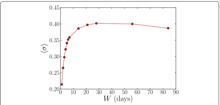
Figure 4 Short-range similarity.The average fraction of linksfcommon to consecutive aggregation windows of durationW.
displays the average similarityσ of networks in consecutive windows of different dura-tionsW. When the windows are very short, the networks are very sparse and the number of common links is low. Then, the similarity increases with increasing window duration, reaching a maximum at∼ days; subsequently, the similarity begins slowly decreasing as the aggregation process captures more and more of the very weak or random links.
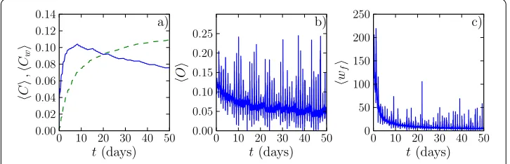
As the growth of the number of links in Figure (b) does not saturate, it is of importance to understand the characteristics of links that emerge early on in the process. It is known from previous investigations [] (with a different set of data) that link weights correlate with the network topology such that high-weight links are associated with dense network neighbourhoods, whereas low-weight links connect such neighbourhoods, in line with the Granovetter hypothesis []. This is directly related to the presence ofcommunity struc-ture[] in social networks; links within communities are stronger and have higher-than-average weights []. For the network aggregation, this means that clusters and commu-nities containing high-weight links are likely to appear early on in the process. In order to investigate this effect, we measure the evolution of the network-level clustering coefficient C(t), given by ×the number of triangles divided by the number of connected triplets in the network. As seen in Figure (a), the clustering coefficient does indeed show a rapid increase as a function of the aggregation interval length, and then decreases after a peak at aroundt= days. This decrease can be attributed to the weak links observed later in the process: those links contribute less frequently to triangles. Hence, if short aggrega-tion periods of around one week are used, the resulting network structure is dominated by strong links associated with dense clusters.
The fact that the edges observed early on in the aggregation process are related to the community structure is also visible when monitoring theoverlap[] of the added links. The overlap of a link connecting nodesiandjis defined as
Oij=nij/
(ki– )+ (kj– ) –nij, ()
Figure 5 Clustering coefficient and topological overlap.(a) Global clustering coefficient of the network and (b) average final overlap of added edges as a function of aggregation time, for the first 2 months. The global clustering coefficient is computed as the number of triangles divided by the number of connected triplets. For the overlap, we calculate the final overlap of edges in the 6-month aggregated network, and average over the final overlap values of newly added links at each time point.
the two connected nodes. Figure (b) displays the average final -month overlap of the added links as a function of aggregation time. Here we have calculated the overlap of each link in the final -month aggregated network, and averaged over these values for links that are added to the network at timet. It is seen that the links that are added early on in the aggregation process have on average a higher overlap than those added later; the final overlap is a decreasing function. Hence, even when the aggregation times are short, the networks capture features of the community structure of the final aggregated networks. Interestingly, the overlap also shows a strong circadian and weekly pattern - its highest peaks correspond to the early morning when the overall call rate is very low. Thus, if calls are made during these hours, they are likely to be targeted towards people in the strongest clusters of friends and family.
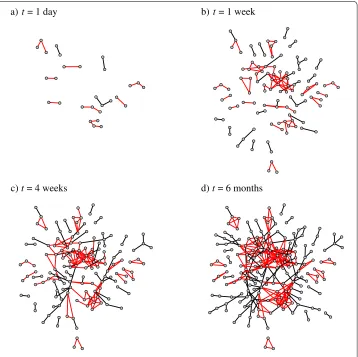
In order to illustrate the network growth, we have visualized small subnetworks corre-sponding to different aggregation timest(Figure ). Here, the subnetwork has been ob-tained by selecting all individuals whose subscriptions are associated with a certain postal code. This method of sampling yields better results than e.g. snowball sampling.a Pan-els (a) to (d) of Figure show the growth of the network, such that edges that participate in triangles in the final -month aggregated network are coloured red. For the shortest aggregation periods (panels (a) and (b)), most of the added edges are in this set, reflecting the above observations on the early appearance of edges connected to communities and clusters. It should be noted that not all community-internal edges are discovered early on; rather, those links that appear early are associated with communities with a high proba-bility.
Behaviour of statistical distributions
under-Figure 6 Aggregated network at different time scales.Series of aggregated networks with a growing aggregation interval. The network aggregated here represents a small subnetwork, obtained by picking individuals from a single postal code. Links that participate in triangles in the final 6-month aggregated network are coloured red, while the rest are black.
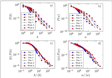
Figure 7 Unscaled and scaled distributions.(a) The degree distribution and (b) the weight distribution for different aggregation intervals, (c) the scaled degree distribution and (d) the scaled weight distribution. The distributions are rescaled with respect to their average value.
f andgdefined over the same domainD⊆Ras
d(f,g) =
D
f(x) –g(x)dx
. ()
To measure the convergence, we have successively calculated the distance between the rescaled degree (weight) distributions of networks aggregated over an interval of length tand networks aggregated over twice longer intervals of length t. In Figure , it is seen
Figure 8 L2distance of rescaled distributions.TheL2distance between the degree (a) and weight (b)
that theLdistance between the degree distributions decreases and converges to a roughly constant value already for aggregation intervals longer than a few days. Hence, already after a short period, a sufficient amount of data has been collected to correctly estimate the stationary degree distribution of the network, and the shape of the degree remains similar for longer intervals. The weight distribution displays a slightly slower convergence, and is still slowly changing even for aggregation intervals of around months; this is also related to the curvature seen in the evolution of the average link weight (Figure (d)). There are several possible explanations for this slower convergence: first, the number of links is increasing and each newly added link brings in a unit of weight. Second, the weights of existing links may display very different time dynamics, and third, the growth of link weights is affected by the burstiness of the call sequences and the resulting long inter-call times. Nevertheless, even the weight distributions do not change much, and care is needed only when interpreting the weight distributions of call networks aggregated over very short periods of time.
On the effects of aggregation window placement
In all analysis so far, we have assumed that the exact placement of the aggregation window, i.e.the time point of its beginning, plays no role in the results. However, as the character-istic daily and weekly patterns of Figure (b) indicate, the overall level of call activity in the network displays large variations by hour and day, and this is expected to have an effect on the aggregated networks, at least on shorter time scales. In addition, there may be less trivial effects if the actual behavioural patterns of individuals - affectingwhothey call - are also time-dependent. In this final section, we will address these issues.
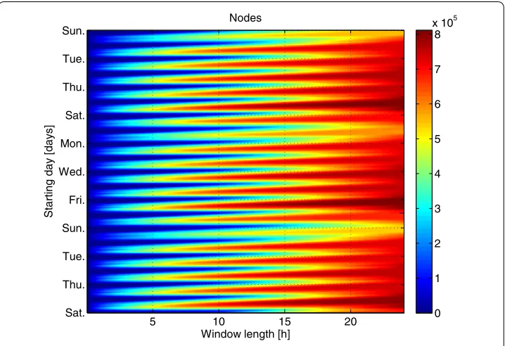
Let us first focus on short time scales, and illustrate the growth of the network with a D heat map plot, displaying the number of nodes in aggregated networks as a function of the aggregation time and the beginning point of the aggregation window (Figure ). The daily and weekly pattern is clearly visible in the plot - the network grows fastest dur-ing weekdays, especially Fridays. The growth is slowest when the aggregation begins on Saturdays and especially Sundays; the difference between Saturdays and Sundays is fairly large. However, this observation might be explained by the network-wide variation of the call frequency alone.
Figure 9 Number of nodes in the network.The number of nodes in the aggregated networks as a function of the aggregation interval length (horizontal axis, in hours) and the beginning point of aggregation (vertical axis). The vertical axis runs from top to bottom, and the first time point is early Sunday, just after midnight.
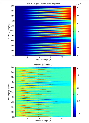
number of nodes in Figure . However, the behaviour of the average giant component size relative to the time-shuffled reference ensemble (lower panel) reveals an interesting feature: when the aggregation begins in the weekends, especially Sundays, the giant com-ponent grows more slowly than it does in the reference. Likewise, for weekdays, it grows far faster than it does in the reference. This points towards different behavioural modes - weekday calls are frequently related to links joining nodes that would otherwise remain disconnected within the aggregation window, whereas weekend calls appear to relate to high-overlap links and dense clusters and thus contribute less to the growth of the largest connected components. In other words, friends and relatives with shared social circles are called more frequently in the weekends.
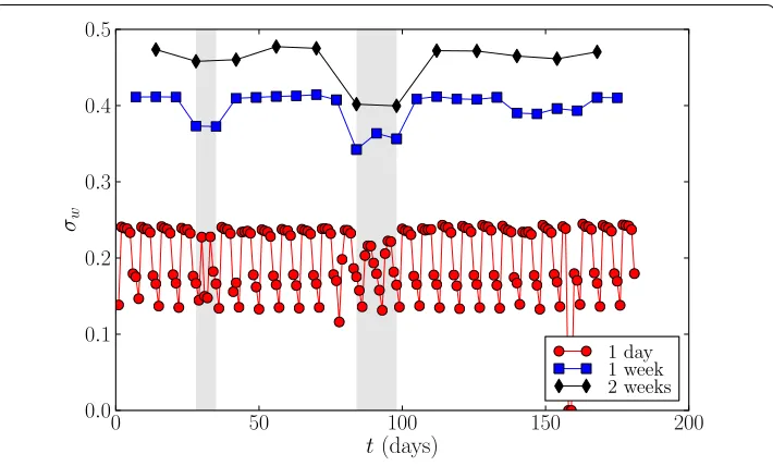
Changes in behaviour very similar to the daily and weekly patterns also appear on longer time scales, as human communication patterns are affectede.g.by holiday periods. In or-der to observe such behavioural changes in the aggregated networks, we divide the data into non-overlapping time windows of day, week, and weeks. We then aggregate net-works corresponding to each time window, and monitor the similarity of the netnet-works in two consecutive windows as a function of time. For this, we employ a weighted general-ization of the Jaccard index of Equation :
σw=
(i,j)∈Emin(wij,wij)
(i,j)∈Emax(wij,wij)
, ()
wherew
Figure 10 Largest connected component size.The absolute (top) and relative (bottom) size of the largest connected component as a function of the aggregation time (horizontal axis) and the beginning point of aggregation (vertical axis). The relative values of the bottom panel are the logarithm of the ratio between the observed largest connected component and the shuffled reference model, where call times do not correlate with network structure.
indi-Figure 11 Long-range similarity.Similarity between networks corresponding to two consecutive aggregation windows of 1 day, 1 week, and 2 weeks. The two shaded areas correspond to national holiday periods: the autumn holiday (left), and holidays around Christmas and New Year (right). The zero-valued points for the 1-day curve are from missing data.
cated by the grey shaded areas. The differences corresponding to holiday periods become much more apparent when aggregation window sizes of week and especially weeks are used, as both measures display a clear drop, especially around the Christmas holiday season. Thus, the calling patterns of individuals are clearly different during such holiday seasons, and this is reflected in the respective aggregated networks that are different from networks aggregated outside the holiday periods.
Conclusions
In many cases, complex networks studied in the literature are constructed by aggregat-ing links or sequences of interactions between the constituent nodes over some period of time, often limited by the availability of data, and their static structural features are then studied. The effects of the aggregation interval length and placement have been discussed only rarely [, ]. In order to shed some insight into this problem, we have investigated the structural features of mobile telephone call networks aggregated over aggregation in-tervals of increasing length. To ensure that the results are not affected by churn,i.e. cus-tomers leaving and subscribing to the operator, we only considered cuscus-tomers whose sub-scriptions did not change over the entire data interval from Oct st, to March th, .
be made. First, because of the broad link weight distribution and Granovetterian weight-topology correlations, where strong links are associated with dense neighbourhoods, the seeds of the underlying community structure are visible in aggregated networks already for rather short aggregation intervals of∼ week: the clustering coefficient of the network peaks at around days, and the earlier a link is observed, the more likely it is to participate in a dense neighbourhood in the final network aggregated over the available data period, as seen by monitoring the neighbourhood overlap of the links. However, at the same time, although the growth of the number of nodes saturates fairly early, the number of links and the average degree of nodes keep on growing even for long aggregation intervals. This sug-gests that for short windows, the cluster and community structures dominate, whereas for longer windows, the contribution of both “weak” links and links that are practically ran-dom,i.e.arise from one-off-calls, increases. When networks from consecutive windows of different lengths are compared, they are seen to be maximally similar at a length of∼ days; this can be considered as the time scale of the recurrent, stable links, beyond which the weaker links start to have a considerable effect on network structure. The scaled de-gree and weight distributions become stationary already for short time intervals of a few days or weeks, respectively.
As the above results are from one dataset only, it is worth considering how general they are. As there are common underlying features of social networks - broad tie strength dis-tributions and the Granovetterian relationship between tie strengths and topology - we believe that the fast emergence of clusters of strong links followed by increasing numbers of weaker links not associated with triangles is a general feature that holds across differ-ent communication networks. Likewise, one may assume that the time scale for obtaining stablest networks (∼ days in our case) should remain roughly similar. However, in both cases, the exact numbers for the characteristic time scales might differ as they may also be affected by the overall call activity level. We also believe that the collapse of scaled distri-butions, indicating stationarity in the underlying processes, should be observable in other data sets too.
In addition to the effects of the aggregation window length, we have shown that com-paring networks aggregated over windows of different placement can yield insight into the dynamic features of the behavioural patterns of individuals. The differences in the growth of the largest connected component point towards different behavioural modes in the weekends and during weekdays, where weekend calls are more frequently related to high-overlap links and dense clusters, and thus build the largest connected compo-nent more slowly; weekday calls play the role of “topological shortcuts” in the aggregation process and more rapidly give rise to overall network connectivity. Additionally, we have observed very different calling patterns during holiday periods, giving rise to aggregated networks that significantly differ from the networks constructed from data outside the holiday periods. Thus, the aggregation interval placement matters, and care should be taken when interpreting the structural features of networks constructed from data that involves holidays or other special periods.
Competing interests
The authors declare that they have no competing interests.
Author’s contributions
Acknowledgements
MK and JS acknowledge financial support of the Future and Emerging Technologies (FET) programme within the Seventh Framework Programme for Research of the European Commission, under FET-Open grant number: 238597 (project ICTeCollective). GK acknowledges support from the Concerted Research Action (ARC) “Large Graphs and Networks” from the “Direction de la recherche scientifique - Communauté française de Belgique”. The scientific responsibility rests with its authors.
Endnote
a Because social networks are geospatially embedded, zip-code-based geospatial sampling yields networks that
preserve rather well the typical characteristics of social networks. On the contrary, in snowball sampling where all nodes at a chosen graph distance from the focal node are included in the sample, the majority of nodes are at the “surface” of the snowball, as the number of nodes grows exponentially with graph distance. This artifact results in low clustering and makes observing community structure difficult.
Author details
1ICTEAM Institute, Université catholique de Louvain, Avenue Georges Lemaître, 4, 1348, Louvain-la-Neuve, Belgium. 2Department of Biomedical Engineering and Computational Science, Aalto University School of Science, P.O. Box 12200, FI-00076, Aalto, Finland.3Swedish Defence Research Agency, SE-147 25 Tumba, Sweden.
Recieved: 7 February 2012 Accepted: 18 May 2012 Published 18 May 2012
References
1. Newman M, Barabási AL, Watts DJ (2006) The structure and dynamics of networks. Princeton University Press, Princeton
2. Newman M (2011) Networks: an introduction. Oxford University Press, Oxford
3. Barrat A, Barthélemy M, Pastor-Satorras R, Vespignani A (2004) The architecture of complex weighted networks. Proceedings of the National Academy of Sciences 101(11):3747-3752
4. Holme P, Saramäki J (2011) Temporal networks. arXiv:1108.1780
5. Holme P (2003) Network dynamics of ongoing social relationships. EPL 64:427
6. Aiello W, Chung F, Lu L (2000) A random graph model for massive graphs. In: Proceedings of the 32nd annual ACM symposium on theory of computing. ACM, New York, pp 171-180
7. Nanavati A, Gurumurthy S, Das G, Chakraborty D, Dasgupta K, Mukherjea S, Joshi A (2006) On the structural properties of massive telecom call graphs: findings and implications. In: Proceedings of the 15th ACM international conference on information and knowledge management. ACM, New York, pp 435-444
8. Seshadri M, Machiraju S, Sridharan A, Bolot J, Faloutsos C, Leskovec J (2008) Mobile call graphs: beyond power-law and log-normal distributions. In: Proceedings of the 14th ACM SIGKDD international conference on knowledge discovery and data mining. ACM, New York, pp 596-604
9. Onnela J, Saramäki J, Hyvönen J, Szabó G, Lazer D, Kaski K, Kertész J, Barabási A (2007) Structure and tie strengths in mobile communication networks. Proceedings of the National Academy of Sciences 104(18):7332
10. Lambiotte R, Blondel V, de Kerchove C, Huens E, Prieur C, Smoreda Z, Van Dooren P (2008) Geographical dispersal of mobile communication networks. Physica A: Statistical Mechanics and its Applications 387(21):5317-5325 11. Onnela J, Saramäki J, Hyvönen J, Szabó G, de Menezes M, Kaski K, Barabási A, Kertész J (2007) Analysis of a large-scale
weighted network of one-to-one human communication. New Journal of Physics 9(6):179
12. Candia J, González MC, Wang P, Schoenharl T, Madey G, Barabási AL (2008) Uncovering individual and collective human dynamics from mobile phone records. Journal of Physics A: Mathematical and Theoretical 41:224015+ 13. Karsai M, Kivelä M, Pan RK, Kaski K, Kertész J, Barabási AL, Saramäki J (2011) Small but slow world: how network
topology and burstiness slow down spreading. Phys Rev E 83:025102
14. Jo HH, Karsai M, Kertész J, Kaski K (2011) Circadian pattern and burstiness in human communication activity. http://arxiv.org/abs1101:0377
15. Krings G, Calabrese F, Ratti C, Blondel V (2009) Urban gravity: a model for inter-city telecommunication flows. Journal of Statistical Mechanics: Theory and Experiment 2009:L07003
16. Blondel V, Krings G, Thomas I (2010) Regions and borders of mobile telephony in Belgium and in the Brussels metropolitan zone. Brussels Studies 42:4
17. Miritello G, Moro E, Lara R (2011) The dynamical strength of social ties in information spreading. Phys Rev E 83:045102(R)
18. Granovetter MS (1973) The strength of weak ties. American Journal of Sociology 78:1360-1380 19. Fortunato S (2010) Community detection in graphs. Physics Reports 486:75-174
20. Tibély G, Kovanen L, Karsai M, Kaski K, Kertész J, Saramäki J (2011) Communities and beyond: mesoscopic analysis of a large social network with complementary methods. Physical Review E 83:056125+
21. Gautreau A, Barrat A, Barthélemy M (2009) Microdynamics in stationary complex networks. Proceedings of the National Academy of Sciences 106:8847-8852
doi:10.1140/epjds4