EOQ Model for Ameliorating Items with Time Dependent Demand and linear Time-Dependent Holding Cost

(1)

Yusuf I. Gwanda, Tahaa Amin, Munkaila Danjuma

Department of Mathematics, Kano University of Science and Technology, Wudil.

Abstract

In many instances, the demand for inventory items fluctuates with time. The demand may increases, decreases, remains constant or even vanishes with time. An economic order quantity model for ameliorating items that describes the above scenario is hereby developed. Stocked items are said to be ameliorative when they incur a gradual increase in quality, quantity or both with time. We develop a model that determines the optimal replenishment cycle time such that the total variable cost is minimized. Numerical examples are given to illustrate the derived model.

Introduction

Demand for inventory items fluctuates with time. The demand for many inventoried items is either periodic, increases, decreases or vanishes with time. In developing countries it is observed that during the harvest period foodstuff flood markets as most of the local farmers stock it in abundance. However as time goes on the stock with some farmers starts getting exhausted and others were forced by daily needs to sale whole or part of their harvest and thus resort to buying food items from the market towards the end of planting session. Hence, the rate of demand for foodstuffs remains partly constant and increases partly with time.

Generally, deterioration is defined as decay, damage, or spoilage which rendered stored items partly or wholly unfit for its original purpose. Food items, chemicals, drugs, electronic components, photographic films, drugs, radio-active substances and so on are some examples

GSJ: Volume 6, Issue 12, December 2018, Online: ISSN 2320-9186

www.globalscientificjournal.com

(2)

The research on deteriorating inventory was pioneered by Ghare and Schrader (1963) who developed a simple economic order quantity model for exponentially decaying inventory. In the course of time, Covert and Philip (1073) extended Ghare and Schrader’s constant deterioration rate to a two-parameter Weibull distribution. Later, Shah and Jaiswal (1997) and Aggarwal (1981) presented and re-established an order level

inventory model with a constant rate of deterioration respectively. Dave and Patel (1981) considered an inventory model for deteriorating items with time-proportional demand when shortages were not allowed. Later, Sachan (1984) extended the model to all for shortages. Hollier and Mak (1983), Hariga and Benkherouf (1994), Wee (1995a, 1995b) developed their models taking the exponential demand. Earlier, Goyal and Giri (2001), wrote an excellent survey on the recent trends in modeling of deteriorating inventory.

The assumption that holding cost is constant at all times is not always realistic as the changes in value of money and price index are dynamic. In this era of globalization where countries engage in tough economic competition, it is unrealistic to assume that holding cost remains constant over time. Various functions describing different forms of holding costs were considered by researchers like Naddor (1966), Van der Veen (1967), Muhlemann and Valtis-Spanopoulos (1980), Goh (1994), Giri and Chaudhuri (1998), and Roy (2008).

Weiss (1982) considered a variation of the economic order quantity model where cumulative holding cost is a nonlinear function of time. The problem involves an approximation of the optimal order quantity for perishable goods, such as milk, and produce, sold in small to medium size grocery stores where there are delivery surcharges due to infrequent ordering, and managers frequently utilize markdowns to stabilize demand as the product’s expiration

date nears. Weiss (1982) showed how the holding cost curve parameters can be estimated via a regression approach from the product’s usual holding cost (storage plus capital costs),

(3)

during t units of time is H(t)=ht, where h and γ ≥ 1 are constants; if γ = 1 then the

problem reduces to the classical EOQ model with h being the cost of holding one unit for one time period. Weiss (1982) also showed in a numerical study that the model provides significant improvement in cost vis-à-vis the classical EOQ model, items with higher daily demand rate, lower holding cost, shorter lifetime, and a markdown policy with steeper discounts.

Tripathi (2013) developed an inventory model for non-deteriorating items under permissible delay in payments in which holding cost is a function of time.

Sharma and Vijay (2013) developed a deterministic inventory model for price dependent demand with time dependent deterioration, varying holding cost and shortages allowed. They assumed that credit limit is available for certain time with no interest, but after that time some interest will be charged.

Karmakar and Choudhury (2014) developed an inventory model for deteriorating items with general ramp-type demand rate, partial backlogging of unsatisfied demand and time-varying holding cost. The authors studied the model under two different replenishment policies, that is, (a) the first replenishment policy starting with no shortages and (b) the second policy starting with shortages. The backlogging rate was assumed to be a non-increasing function of the waiting time up to the next replenishment.

(4)

items (in the farm) undergo increase in quantity and quality. The items that exhibit such properties are referred to as ameliorating items.

The ameliorative nature of inventory was not given much attention until recently. Hwang (1997) developed an economic order quantity model (EOQ) and partial selling quantity model (PSQ) for ameliorating items under the assumption that the ameliorating time follows the Weibull distribution. Again, Hwang (1999, 2004) developed more inventory models for both ameliorating and deteriorating items separately under the LIFO and FIFO issuing policies. Later Moon et al (2005) developed an EOQ model for ameliorating/deteriorating items under inflation and time discounting. The model studied inventory models with zero-ending inventory for fixed order intervals over a finite planning horizon allowing shortages in all but in the last cycle. They also developed another model with shortages in all cycles taking into account the effects of inflation and time value of money. A partial selling inventory model for ameliorating items under profit maximization was studied by Mandal et al (2005).

In our present study, we focus our attention on ameliorating inventory where the rate of amelioration is constant but the demand is linearly dependent on time.

Assumptions and Notation

The proposed ameliorating inventory model is developed under the following assumptions and notation:

The inventory system involves only one single item.

Amelioration occurs when the items are effectively in stock.

The cycle length is T.

(5)

The inventory carrying cost in a cycle is .

The unit cost of the items know constant C And the replenishment cost is also a constant

per replenishment.

The demand rate per unit time R is dependent on time.

The total demand in a cycle is

The rate of amelioration A is constant.

The ameliorated amount when considered in items of value (say weight) in a cycle is

Inventory ordering charge per unit i, is a known constant.

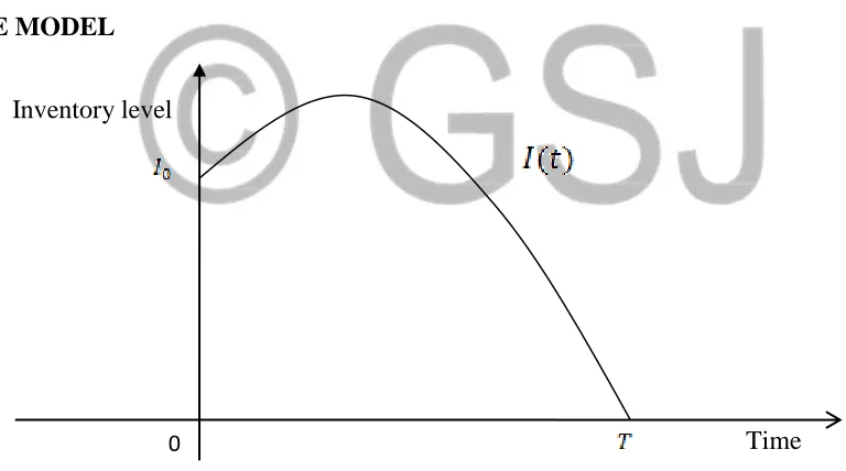
THE MODEL

Inventory level

Time

Fig 1: inventory movement with an ameliorating inventory system with time depended demand

During the time interval amelioration occurs at a constant rate A and the

demand rate is time dependant. The differential equation that describes the instantaneous state of inventory level I(t) is given by

(6)

 

I t AI t bt dt

d

− =

− ( )

)

( (1)

The solution of the above equation is given by:

At ke b Abt A t

I( )= 1₂ ( + )+ (2)

Where k is a constant.

Applying the boundary condition at and substituting these values in

equation (2) yields

k A

b

I = +

2

0

So that ₀ ₂

A b I

k = − (3)

Substituting equation (3) into equation (2), we obtain;

At At

e I e At A

b t

I( )= ₂( +1− )+ ₀ (4)

Also when t = T, I(t) = 0. Hence equation (4) becomes-

AT AT

e I e AT

A b

0

2( 1 )

0= + − +

) 1 ( 2 0

AT AT

e AT A

b e

I =− + −

2 2

0 ( 1)

A b e

AT A

b

I =− + −AT +

(7)

Substituting equation (5) into equation (4) gives:

At AT

At

e A

b e

AT A

b e

At A

b t I

  

₋ ₊ ₊

+ − +

= −

2 2

2( 1 ) ( 1)

) (



( )



2 ( 1) ( 1)

T t A e AT At

A

b ₊ ₋ ₊ −

= (6)

From Appendix I the total demand within the time interval is obtained as:

2 2

bT RT =

(7)

From Appendix II the ameliorated amount is given by;

2 2

2

) 1 (

2 A

b e

AT A

b bT

A_m = + + −AT −

(8)

From Appendix III the linearly time dependent holding cost in the period, is given by;







2 3 6 6 6



6 2 2

2 2

)

( 2 2 ₄2 3 3 2 2

3

1 + + − + − − − +

= −AT −AT −AT −AT

h AT A T ATe e

A bCi e

ATe T

A A bCi t

C  

(9) Total variable cost per unit time in a cycle,(TVC(T))=Inventory Ordering cost+ Holding cost- Cost of Ameliorated Amount that is

) (

1 )

( ₀

m A

h C

C C T T

(8)









                          − + + −     ₋ ₋ ₋ ₊ +     ₊ ₊ ₊ ₋ = − − − − − 2 2 2 2 2 3 3 4 2 2 2 3 1 0 ) 1 ( 2 6 6 6 3 2 6 1 2 2 2 2 1 ) ( A b e AT A b bT T C e ATe T A T A A bCi T e ATe T A A bCi C T T TVC AT AT AT AT AT



                          − + + −       + − − − +       − + + + = − − − − − − T A b T A be A be bT C T T e Ae T A T A A bCi T T e Ae T A A bCi T C AT AT AT AT AT AT 2 2 2 2 3 4 2 2 3 1 0 2 6 6 6 3 2 6 2 2 2 2   (10)

Equation (10) is then differentiated with respect to T to obtain

(9)

                          + + − − −       − + + − − +       + + − − + − = − − − − − − 2 2 2 2 2 2 2 2 3 4 2 2 2 2 2 3 1 2 0 ) 1 ( 2 6 ) 1 ( 6 6 3 4 6 2 ) 1 ( 2 2 2 T A b T A e AT b be b C T T e AT e A A T A A bCi T T e AT e A A A bCi T C AT AT AT AT AT AT   (11)

For optimal T which minimizes the total variable cost per unit time, we have



( )



=0

dT T TVC d

provided





dT T TVC

d ( )

That is;                           + + − − −       − + + − − +       + + − − + − = − − − − − − 2 2 2 2 2 2 2 2 3 4 2 2 2 2 2 3 1 2 0 ) 1 ( 2 6 ) 1 ( 6 6 3 4 6 2 ) 1 ( 2 2 2 T A b T A e AT b be b C T T e AT e A A T A A bCi T T e AT e A A A bCi T C AT AT AT AT AT AT  

This simplifies to;

(

)

(

)





_                + + − − − − + + − − + + + − − + − = − − − − − − 2 ) 1 ( 2 2 2 6 ) 1 ( 6 6 3 4 6 2 ) 1 ( 2 2 2 0 2 2 2 2 2 2 2 2 2 2 3 3 2 4 2 2 2 2 2 2 3 1 2 0 AT AT AT AT AT AT e AT e T A T A T A Cb e AT e T A T A T A T A bCi e AT e T A T A T A bCi T C  

(

)

(

)





         + + − − − − + + − − + + + − − + − = − − − − − − 2 ) 1 ( 2 2 3 6 ) 1 ( 6 6 3 4 2 ) 1 ( 2 2 3 6 2 2 2 2 2 2 2 2 2 3 3 2 2 2 2 2 1 0 4 AT AT AT AT AT AT e AT e T A T A Cb A e AT e T A T A T A bCi e AT e T A T A AbCi C A   (12)

However from equation (5), (7) and (8) we have

m

t A

R I

EOQ= ₀ = −

(

AT

)

e AT A

b ₋ ₊ −

= ₂ 1 ( 1)

(10)

Numerical examples:

The table below gives the solutions of ten different numerical examples with different parameters, using equations (12) and (13). In all the ten cases, the value

, 0 )] ( [ 2 2

 T TVC dT

d

and so the solutions are for minimum values

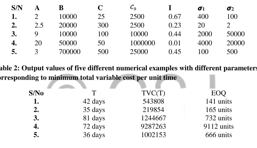
Table 1: Input values of five different numerical examples with different parameters corresponding to minimum total variable cost per unit time

S/N A B C I 𝞼1 𝞼2

1. 2 10000 25 2500 0.67 400 100

2. 2.5 20000 300 2500 0.23 20 2

3. 9 10000 100 10000 0.44 2000 50000

4. 20 50000 50 1000000 0.01 4000 20000

5. 3 700000 500 25000 0.45 100 500

Table 2: Output values of five different numerical examples with different parameters corresponding to minimum total variable cost per unit time

S/No T TVC(T) EOQ

1. 42 days 543808 141 units

2. 35 days 219854 165 units

3. 81 days 1244667 732 units

4. 72 days 9287263 9112 units

5. 36 days 1002153 666 units

Sensitivity analysis

We then carry out a sensitivity analysis on the first example to see the effect of parameter changes on the decision variables. This has been done by changing the parameters by 1%, 5%, and 25% and taking one parameter at a time, keeping the remaining parameters constants.

(11)

Table 3: Sensitivity analysis to see the effect of percentage change in the rate of amelioration, A, on decision variables

b= 10000, C = 25, C0 = 2500, i = 0.67, 𝞼1 = 400, 𝞼2 =100 % change in

the value of A

% change in results *

T TVC(T*) EOQ

-25 -5 8 -16

-5 -3 2 -4

-1 0 0 1

1 1 0 2

5 2 -2 4

25 9 -9 25

From Table 3, we can see that T and EOQ increase with increase in A, but TVC(T) decreases. Such phenomenon implies that the higher the rate of amelioration, the higher the rate of accumulation of the inventory and hence, the higher the EOQ and the longer the period it takes to dispose it. The total variable cost decreases as expected since the high rate of amelioration alleviates the invested costs.

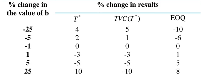
Table 4: Sensitivity analysis to see the effect of percentage change in the rate of demand, b, on decision variables

A= 2, C = 25, C0 = 2500, i = 0.67, 𝞼1 = 400, 𝞼2 =100 % change in

the value of b

T TVC(T*) EOQ

-25 4 5 -10

-5 2 1 -6

-1 0 0 0

1 -3 -3 1

5 -5 -5 5

25 -10 -10 8

(12)

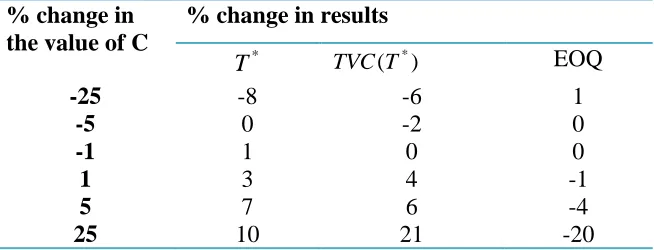
Table 5: Sensitivity analysis to see the effect of percentage change in the unit cost of items, C, on decision variables

A = 2, b = 10000, C0 = 2500, i = 0.67, 𝞼1 = 400, 𝞼2 =100 % change in

the value of C

T TVC(T*) EOQ

-25 -8 -6 1

-5 0 -2 0

-1 1 0 0

1 3 4 -1

5 7 6 -4

25 10 21 -20

Table 5 shows that all the decision variables are sensitive to change in the cost of items. As the unit cost of items soars high, it invariably induces increase in other costs resulting in low demand and thus elongates the cycle period and hence, a low EOQ.

Table 6: Sensitivity analysis to see the effect of percentage change in the ordering cost, C0, on decision variables

A = 2, b = 10000, C = 25, i = 0.67, 𝞼1 = 400, 𝞼2 =100 % change in

the value of C0

T TVC(T*) EOQ

-25 -7 23 12

-5 0 3 0

-1 0 1 0

1 2 -3 -4

5 2 -6 -4

25 11 -19 -22

The tabulated results above conform to the theoretical aspect of Inventory which asserts that the high rate of ordering cost reduces the frequency of placing orders and hence, results in a reduced TVC(T) and EOQ.

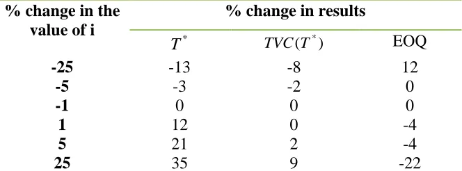
Table 7: Sensitivity analysis to see the effect of percentage change in the inventory holding charge, i, on decision variables

(13)

% change in the value of i

T TVC(T*) EOQ

-25 -13 -8 12

-5 -3 -2 0

-1 0 0 0

1 12 0 -4

5 21 2 -4

25 35 9 -22

In conformity with real life, a high inventory holding charge results in high TVC(T), an elongated T* (since this will induce increase in selling price which in turn will reduce the demand rate and hence elongates the rate of depletion of the items) and a low EOQ as illustrated by the Table above.

Table 8: Sensitivity analysis to see the effect of percentage change in the initial holding cost, 𝞼1, on decision variables

A = 2, b = 10000, C = 25, C0 = 2500, I = 0.67, 𝞼2 =100 % change in the

value of 𝞼1

T TVC(T*) EOQ

-25 -8 -43 22

-5 -5 -27 10

-1 0 8 2

1 2 0 -4

5 7 2 -7

25 18 9 -27

A high initial holding cost results in high TVC(T) and low EOQ and an elongated T* as illustrated by the Table above.

Table 9: Sensitivity analysis to see the effect of percentage change in the trend in holding cost, 𝞼2, on decision variables

A = 2, b= 10000, C = 25, C0 = 2500, I = 0.67, 𝞼1 =400 % change in the

value of 𝞼2

T TVC(T*) EOQ

-25 -7 -7 10

-5 0 -3 5

-1 0 0 0

1 2 2 -1

5 5 2 -6

(14)

(15)

Reference

Aggarwal, S.C., (1981), Purchase-inventory decision models for inflationary conditions, Interfaces 11 18–23.

Covert, R.P. and Philip, G.C., (1973), An EOQ Model for Items with Weibull Distribution,

AHE Trans 5(4), 323-326

Dave, U. and Patel, U.K., (1981). (t,Si) policy inventory model for deteriorating items with time proportional demand. J. of Opl.Res.Soc., 32: 137-142

Ghare, P.M. and Shrader, G.F., (1963), A Model for Exponential Decaying Inventory,

Journal of Industrial Engineering 14: 238-243

Giri, B.C., Chaudhuri, K.S., (1998): Deterministic models of perishable inventory with stock-dependent demand rate and non-linear holding cost, European Journal of Operational Research, 105(3), 467-474.

Goh, M., (1994): EOQ models with general demand and holding cost functions,

European Journal of Operational Research,73,50-54.

Goyal S.K. and Giri B.C. (2001), Recent trends in modeling of deteriorating inventory, European Journal of Operational Research 134(1) 1-16

Hariga, M.A., and Benkherouf, L., (1994). Optimal and heuristic inventory replenishment models for deteriorating items with exponential time varying demand. European J. of Operational Research, 79: 123-137

(16)

Hwang S.K., (1997), A study of Inventory model for items with Weibull ameliorating,

Computers and Industrial Engineering, 33: 313-325

Hwang S.K. (1999), Inventory models for both ameliorating and deteriorating items,

Computers and Industrial Engineering, 37: 257-260

Hwang, H.S., Kim, H.G. and Paik, C.H., (2005), Optimal Issuing Policy for Fish-Breeding Supply Center with Items Weibull Ameliorating, International Journal of the Information Systems for Logistics and Management 1(1,) pp. 1-7

Karmakar, B., Choudhury, K.D., (2014), Inventory models with ramp-type demand for deteriorating items with partial backlogging and time –varying holding cost, Yugoslav Journal of Operation Research, 2: 249-266

Mondal B., Bhunia A. K. and Maiti M. (2003), An inventory system of ameliorating items for price dependent demand, Computers and Industrial Engineering,45: 443-456.

Moon I., Giri B. C. and Ko B. (2005), Economic order quantity model for ameliorating/deteriorating items under inflation and time discounting, European Journal of Operations Research 173(2) 1234-1250.

Moon I., Giri B. C. and Ko B. (2006), Erratum to ‘‘Economic order quantity model for ameliorating/deteriorating items under inflation and time discounting’’ European Journal

of Operations Research 174(2) 1345-1347.

Muhlemann, A.P. and Valtis-Spanopoulos, N.P., (1980), A variable holding Cost rate EOQ model, European Journal of Operational Research, 4 132-135

(17)

Roy, A., (2008), An inventory model for deteriorating items with price dependent demand and time varying holding cost, Advanced modeling and optimization, 10(1):25-37

Sachan, R.S., (1984): On (T, Si) policy inventory model for deteriorating items with time proportional demand, Journal of the Operational Research Society, 35: 1013-1019.

Shah, Y.K. and Jaiswal, M.C.,(1997), An order-level inventory model for a system with constant rate of deterioration, Opsearch 14: 174–184.

Sharma, S.C., Vijay, V., (2013), An EOQ Model for Deteriorating Items with Price Dependent Demand, Varying Holding Cost and Shortages under Trade Credit,

International Journal of Science and Research, Volume 4(1) 445-438.

Tripathi, R.P., (2013), Inventory model with cash flow oriented and time-dependent holding cost under permissible delay in payments, Yugoslav Journal of Operation Research, JIEC,

4(1): 122-132.

Van Der Veen, B., (1967): Introduction to the theory of Operational Research, Philip Technical Library, Springer-Verlag, New York.

Wee, H.L., (1995a), A deterministic lot-size inventory model for deteriorating items with shortages and a declining market, Compt. Operat. Res., 26: 545-558

Wee, H.L., (1995b), Joint Pricing and Replenishment Policies for Deteriorating Inventory with declining markets, International Journal of Production Economics, 40: 163-171

(18)

Appendix I: The total demand within the time interval is obtained as: 2 2 2 0 2 0 bT t b btdt R T T T = = =

_

(7)

Appendix II: The ameliorated amount within the interval is obtained as:

A_m =R_T −I₀

   ₋ ₊ ₊ − = − 2 2 2 ) 1 ( 2 A b e AT A b bT AT ₂ ₂ 2 ) 1 ( 2 A b e AT A b

bT + + AT −

= −

Appendix III: The linearly time dependent holding cost in the period, is obtained as:

C_h(t) iC T( t)I(t)dt

0 1 2



+

=  



At AT e



dt

A b t iC

t

C_h T At T

    ₊ ₋ ₊ + = −



( ) 2

0 ( 1 2 ) ( 1) ( 1) )

(  





_







₊ ₋ ₊ − ₊ ₊ ₋ ₊ −

= T At T T At T

h t At AT e dt

A bCi dt e AT At A bCi t C 0 ) ( 2 2 0 ) ( 2

1 ₍ ₁₎ ₍ ₁₎ ₍ ₁₎ ₍ ₁₎

) (               − − + + − − + =



− − − − dt te A bCi dt te A bCTi tdt A bCi dt t A bCi dt e A bCi dt e A bCTi dt A bCi dt t A bCi T T t A T T t A T T

T _A_t _T T _A_t _T

(19)

. 1 1 2 3 1 1 2 2 2 2 2 2 2 2 2 2 2 3 2 2 1 1 2 1 2 1                     + − −       + − − + +       − −       − − + = − − − − A e A A T A bCi A e A A T A bCTi A T bCi A T bCi A e A A bCi A e A A bCTi A T bCi A T bCi AT AT AT AT                     − + − − + − + + − + = ₋ ₋ − − 4 2 4 2 3 2 3 2 3 2 2 2 2 3 2 3 1 3 1 2 1 2 1 2 3 2 A e bCi A bCi A bCTi A e bCTi A bCTi A T bCi A T bCi A e bCi A bCi A e bCTi A T bCi AT AT AT AT           







2 3 6 6 6



6 2 2 2 2 2 2 3 3 4 2 2 2 3

1 + + − + − − − +

= −AT −AT _A_T _A _T _ATe−AT _e−AT

A bCi e ATe T A A