https://doi.org/10.5194/npg-25-649-2018 © Author(s) 2018. This work is distributed under the Creative Commons Attribution 4.0 License.
Climatic responses to systematic time variations of parameters:
a dynamical approach
Catherine Nicolis
Institut Royal Météorologique de Belgique, 3 av. Circulaire, 1180 Brussels, Belgium Correspondence:Catherine Nicolis ([email protected])
Received: 18 April 2018 – Discussion started: 28 May 2018
Revised: 1 August 2018 – Accepted: 20 August 2018 – Published: 4 September 2018
Abstract.The climatic response to time-dependent parame-ters is revisited from a nonlinear dynamics perspective. Some general trends are identified, based on a generalized stabil-ity criterion extending classical stabilstabil-ity analysis to account for the presence of time-varying coefficients in the evolution equations of the system’s variables. Theoretical predictions are validated by the results of numerical integration of the evolution equations of prototypical systems of relevance in atmospheric and climatic dynamics.
1 Introduction
The climatic impact of systematic variations of certain key parameters in time arising from anthropogenic effects such as increasing CO2concentration constitutes currently a ma-jor scientific, economic and societal issue (Goodie and Guff, 2001). There exists a vast literature on the subject culminat-ing in the derivation of a number of scenarios of future cli-matic change, based on the integration of detailed numerical models and on the intercomparison of their respective pre-dictions (Andrews et al., 2012).
On the other hand, it is widely recognized that the atmo-sphere and climate are highly nonlinear systems subjected to intricate feedbacks giving rise to a rich variety of com-plex dynamical behaviors such as self-generated periodic-ities, deterministic chaos, or transitions between different states (Nicolis and Nicolis, 1987; Dijkstra, 2013). A major advance of nonlinear dynamics has been to show that these behaviors often rest on a limited number of generic, global features independent of details concerning individual pro-cesses (Guckenheimer and Holmes, 1983). This suggests that it might be of interest to search for regularities likely to
re-cur across different models and scenarios that could possi-bly be masked in a detailed full-scale analysis. In this work we revisit the climatic response to time-dependent parame-ters from such a nonlinear dynamics perspective, extending an early investigation in this direction by the present author (Nicolis, 1988).
The starting point is a set of equations governing the evo-lution of the atmospheric and climatic variables. We consider a reference state corresponding to a solution of these equa-tions for some particular values of the parameters. We next switch on a systematic variation of these parameters in time and follow the subsequent transient response of the reference state to this forcing. The questions we raise are whether and if so for how long the system will follow passively this varia-tion while remaining in the same branch of states; under what conditions it will jump to a new regime and if so when this transition will occur; and finally, whether states that would otherwise prevail in the absence of parameter variation are altered significantly or missed altogether.
A general formulation for addressing these questions is outlined in Sect. 2, where a generalized stability criterion for remaining or not in the vicinity of the reference state is de-rived and some general scenarios of subsequent evolution are discussed. In the light of these ideas the response to time-varying parameters is analyzed in Sects. 3 to 5 in situations giving rise to oscillatory behavior, to chaotic behavior and to transitions between simultaneously stable states. The main conclusions are summarized in Sect. 6.
2 Formulation
Let{xi},i=1,· · ·, nbe the set of atmospheric/climatic
vari-ables andλα,α=1,· · ·, r a set of parameters characteristic
of the rates of the various processes involved in the evolution of these variables. The rate of change of{xi}in time will be
given by a set of equations of the form dxi
dt =Fi {λα},{xj}
, i, j=1,· · ·, n, (1) where the evolution laws{Fi}are, typically, nonlinear
func-tions of the{xj}.
We are interested in situations in which one of these pa-rameters varies systematically in time as a result of an ex-ternally induced forcing of natural or anthropogenic origin. The particular form of variation we shall focus on is a slow variation in the form of a ramp,
λ(t )=λ0+t, 1, (2)
wheretis the time andλ0the value ofλprevailing at a stage where the evolution of the {xi} is started. Introducing the
slow timescale
τ =t, (3a)
one may cast Eqs. (1) in the form
dxi
dτ =Fi λ(τ ),{xj}
, (3b)
where from now on we will discard all parameters other than the time-varying oneλ(τ ).
Following the procedure outlined in the Introduction we consider now a particular, possibly time-dependent state{xi}
lying at t=0 on an invariant attracting set of states corre-sponding to the valueλ0of parameterλand switch on next the change of λin time according to Eq. (2). We are inter-ested in the response of the reference state{xi}to this change
as defined by the instantaneous deviations from it,{δxi},
ini-tially assumed to be small. Writing
xi=xi+δxi (4a)
and substituting into Eq. (3b), one obtains then a linearized set of equations of the form
dδxi
dτ =
X
j
Jij(τ )δxj, (4b)
where Jij= ∂Fi/∂xj{x
j} are the elements of the
Jaco-bian matrix associated to Fi. These quantities depend on τ through the time dependence of λ (Eq. 2) and possibly through the fact that the reference state{xi}may itself be part
of a periodic or chaotic attractor. In what follows we will be especially interested in the dependence onτ induced byλ.
Equations (4b) constitute a set of coupled equations with slowly varying coefficients. Generalizing the time-exponential solutions familiar from classical stability anal-ysis, we seek solutions of these equations of the WKB form (Kevorkian and Cole, 1996):
δxi(τ )=exp 1
8(τ )
Ai(, τ ), (5)
where the amplitudesAi depend smoothly on. Substituting
into Eqs. (4b) we obtain, to the dominant order in,
Ai
d8
dτ =
X
j
Jij(τ )Aj.
It follows that the quantity
w(τ )=d8
dτ (6a)
satisfies the generalized characteristic equation
det|Jij(τ )−w(τ )δijkr| =0 (6b)
and plays thus the role of a generalized eigenvalue of the (time-dependent) Jacobian matrixJ(τ ).
We are now in the position to derive the condition under which the response{δxi(τ )}will remain bounded or will, on
the contrary, show explosive behavior. Taking Eq. (5) into ac-count one sees straightforwardly that the threshold separating these two regimes is given by the relation
Re8(τc)=
τc Z
0
dτ0Rew τ0=0. (7)
This relation, if satisfied, defines a critical timetc=τc and a corresponding critical valueλc=λ0+tcof parame-terλbeyond which the system will depart from the reference state and evolve toward a new branch of solutions. We expect that these solutions will be part of the bifurcation diagram of the dynamical system defined by Eqs. (1). The question will then be how these solutions are reached if one moves across this bifurcation diagram according to Eq. (2), starting from a stable branch of solutions. In particular, are the transitions toward the new states taking place in the “static” bifurcation points of Eq. (1), and if not, in the “dynamical” view of bi-furcation adopted here, are the transitions advanced, delayed or skipped altogether (Erneux and Mandel, 1986; Baer et al., 1989; Benoit, 1991; Nicolis and Nicolis, 2004, 2014). Failure to satisfy relation (7) for anyτ within a certain range, start-ing atτ=0 from a stable branch of solutions, would on the other hand imply that the system will remain on this branch of solutions for this time period. One would then like to know how the structure of this solution is affected as the parameter
system to cross threshold values that would otherwise never be reached.
In what follows these questions will be addressed for se-lected classes of systems giving rise to periodic behavior, to chaotic dynamics and to transitions between simultane-ously stable steady states. We stress that the logic under-lying our formulation differs from the one adopted in typ-ical general circulation model-based experiments (Gregory et al., 2015) in which, e.g., CO2 concentration is suddenly increased (CMIP5 abrupt n×CO2 experiments wheren is typically 2 or 4) and the system is subsequently left to relax to its final state, keeping this concentration constant.
3 Periodic behavior
A dynamical system giving rise to sustained oscillations must involve at least two coupled variables. The onset of oscilla-tory behavior will occur through a Hopf bifurcation, in the vicinity of which the Jacobian matrix associated to the rate functions{Fi}in Eqs. (1) possesses two complex conjugate
eigenvalues whose real parts become positive beyond the bi-furcation point (Guckenheimer and Holmes, 1983). An in-teresting example of Eqs. (1) of relevance in climate theory giving rise to this type of behavior is the sea ice–ocean sur-face temperature model developed by Saltzman, Sutera and Hansen (Saltzman et al., 1982) which in appropriate rescaled variables reads as (Nicolis, 1984)
dη
dt = −η+θ,
dθ
dt = −aη+bθ−η
2.θ (8)
Hereηrepresents the deviation of the sine of the latitude of sea ice extent from the reference steady state and θ the excess mean ocean surface temperature.aandbare positive parameters describing, respectively, the negative feedback of ice extent on temperature and the positive feedback of tem-perature on itself. Finally,η2θaccounts for nonlinear restor-ing mechanisms.
Previous studies have shown that as long as a > b the steady-state solutionη=θ=0 of Eqs. (8) is stable for values of the parameterbless than 1 and loses its stability through a Hopf bifurcation toward time-periodic solutions at a critical valueb(c0)=1.
In the context of the present work it will be natural to choosebas the time-dependent parameter
b=b0+t. (9)
We choose again as a reference state the steady-state solu-tionη=θ=0 and a starting valueb0for which this state is stable (b0<1) and seek solutions of Eq. (8) when the time dependence ofb is switched on according to Eq. (9) in the WKB forms of Eq. (5). One obtains then straightforwardly
the following explicit form of the generalized characteristic equation (Eq. 6b):
d8
dτ
2
−(b0+τ−1) d8
dτ +(a−(b0+τ ))=0, (10)
where we have again setτ =t. In view of our choiceb0<1 anda > bthere exists a range of values ofτ for which this equation admits complex conjugate roots: (d8/dτ )±. The
stability criterion expressed by Eq. (7) in terms of the real part of these solutions leads then to the explicit form
Re8±(τc)=
τc Z
0 dτ0Re
d8 dτ0
=1 2
τc Z
0
dτ0 b0−1+τ0
=1 2
(b0−1) τc+
τc2 2
=0. (11)
This relation determines a critical time
tc=
2(1−b0)
(12a)
and a new critical parameter value
bc=b0+tc=2−b0 (12b)
independent of , beyond which the system will leave the reference state and evolve toward a periodic solution. The point is that (a), unlessb0=1,bcis different from the value
b(c0)=1 corresponding to the “static” Hopf bifurcation point, and (b), as a result the transition to the instability region is postponed for a time interval proportional to the distance of
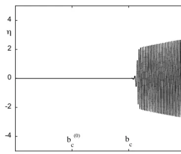
b(c0) from the starting valueb0and inversely proportional to the smallness parameter. During this delay the system will keep following the initial branch of states, which in the clas-sical setting of time-independent parameterbwould be un-stable and is now temporarily stabilized. In a climate dynam-ics perspective one could rephrase this result by the state-ment that rather than precipitating the system to the insta-bility that was bound to occur atb(c0)=1 and to the large deviations in the form of oscillations that would follow, the time-dependent forcing has on the contrary postponed this “catastrophe”. Everything happens as if the presence of the time-dependent forcing during the time spent in the stable region enhances the “inertia” of the system and hence its fur-ther stabilization into this region. This realization illustrates how long-term predictions can interfere in a subtle and unex-pected manner with the dynamical complexity of the under-lying system.
-4 -2 0 2 4
0 1 2 b
b
c
(0)
b
c
Figure 1.Evolution of variableηversus the instantaneous value of
the feedback parameterbas obtained numerically from model (8) in the presence of a time dependenceb=b0+twithb0=0,a=4
and=0.01.
according to Eq. (9). Figure 1 depicts the evolution of vari-ableηin a representation where time enters through the pa-rameterb=b0+t, witha=4,b0=0 and=0.01. As can be seen the system follows the stateη=0, runs across the static Hopf bifurcation pointb(c0)=1 as if nothing was hap-pening and finally jumps to an oscillatory state at a time cor-responding to b=2, in full agreement with the theoretical result of Eqs. (12a) and (12b). On the other hand, when the transition is finally taking place the system is rapidly precipi-tated in a regime of large-amplitude oscillations, much larger than those that would start smoothly atb(c0)=1 in the classi-cal setting of a static Hopf bifurcation. We witness, in some sense, a payoff between the postponement and the extent of a potentially catastrophic event.
These results hold for a wide range of values of , but at some point one witnesses deviations from the asymptotic regime as captured by the WKB type of solutions. The trend, as illustrated in Fig. 2, is that for increasing(here=0.1) the transition to oscillations is further postponed beyond the value predicted by our theoretical estimate. We conjecture that this is due to the fact that the bifurcation diagram is now traversed faster than the characteristic growth rates of perturbations that would otherwise remove the system from the reference state. These perturbations are thus temporarily quenched until their growth rate becomes substantial and can no longer be counteracted by moving across the bifurcation diagram.
A question related to the foregoing observations and of in-terest in the context of atmospheric and climate dynamics is when a particular variable of relevance in a system subjected to a systematic time-dependent forcing will cross for the first time a certain prescribed level. Figure 3 summarizes the re-sults obtained by numerically integrating Eqs. (8) and (9) for a wide range of values of the ramp parameter and for a threshold value|η| =1 set for the variableηof the model. We
-4 -2 0 2 4
0 1 2 3 4 5 6 b
b c
(0) b
c
Figure 2.As in Fig. 1 but=0.1.
2 2.5 3
0 0.02 0.04 0.06 0.08 0.1 b
Figure 3.Instantaneous value of parameterbcorresponding to the
first passage of variableηfrom threshold|η| =1 versus the intensity
of the ramp parameter withb0=0. Other parameter values as in Fig. 1.
observe an ascending trend with increasingvalues, which can be explained qualitatively by the arguments advanced in connection with Fig. 2.
4 Chaotic dynamics
(vari-ablesyandz). One arrives then at the equations dx
dt =σ (−x+y),
dy
dt =rx−y−xz,
dz
dt =xy−bz. (13)
The parametersσ andr are scaled Prandtl and Rayleigh numbers, respectively, and b accounts for the geometry of the convective pattern.
Equations (13) have been studied extensively in the litera-ture (Sparrow, 1982). We briefly summarize some results that will be relevant for our purposes.
– (i) The steady statex=y=z=0 (where convection is absent) is stable forr <1 and loses its stability atr=1 through a pitchfork bifurcation.
– (ii) Beyondr=1 a pair of non-trivial steady states rep-resentative of convection emerges, given byx±=y±=
±√b(r−1),z=r−1. These states remain stable forr
less than a threshold valuerT(0)=σ (σ+b+3)/(σ−b− 1).
– (iii) Atr=rT(0)a Hopf bifurcation is occurring, but the branches of periodic solutions are subcritical (i.e., exist forr < rT(0)) and thus unstable.
– (iv) Beyond rT(0) one observes a variety of complex chaotic behaviors which emerge suddenly as global, finite-amplitude solutions.
In what follows it will be natural to considerr, which in-corporates the effect of the thermal constraints acting on the system, as a time-dependent parameter.
Setting
r=r0+t (14)
we choose as the reference state one of the convective states, say (x−,y−,z), and a starting valuer0for which this state is stable, i.e., 1< r0< rT(0). Similarly to Sect. 3 we seek solutions of Eqs. (13) with time-dependent r according to Eq. (14) in the WKB form of Eq. (5). We obtain in this way the following explicit form of the generalized characteristic Eq. (6) associated to the Jacobian matrix of Eqs. (13) around (x−,y−,z):
d8 dτ
3
+(σ+b+1)
d8 dτ
2
+b (σ+r0+τ ) d8
dτ
+2bσ (r0+τ−1)=0, (15) whereτ =t. The system will leave the reference state at a critical timetc=τc/and a critical,-independent parameter
25 30 35 40
10 15 20 r 25
0 r
c
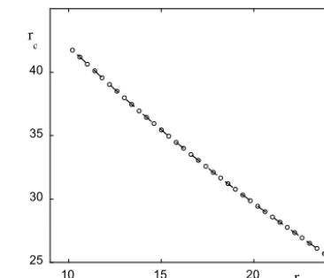
Figure 4.Theoretical estimate of the onset of chaotic solutions
ver-sus the initial value of parameterr0 (Eq. 15) for model (13) in
the presence of a time dependence in the form ofr=r0+twith =0.01. Other parameter values areσ=10 andb=8/3.
valuerc=r0+tcdetermined by relation (7),
Re8 (τc)=
τc Z
0 dτ0Re
d8 dτ0
=0, (16)
where d8/dτ as a function ofτ is given by Eq. (15). Figure 4 summarizes the results obtained by numerical evaluation of the integral in Eq. (16). We have set for this pur-poseσ=10,b=8/3 in Eq. (15). The static Hopf bifurcation pointrT(0)corresponding to these values isrT(0)≈24.74. We chooser0values in the interval (10, 24) prior to this value, for which Eq. (15) in the absence of a time-dependent pa-rameter possesses a real negative root and a pair of complex conjugate roots with a negative real part. We then plot in the figure the critical value ofrof the onset of chaotic solutions,
rc=r0+τc, as a function ofr0. As can be seenrcdecreases quasi-linearly withr0, from a value of about 45 atr0=10 to a value of about 25.5 atr0=24.
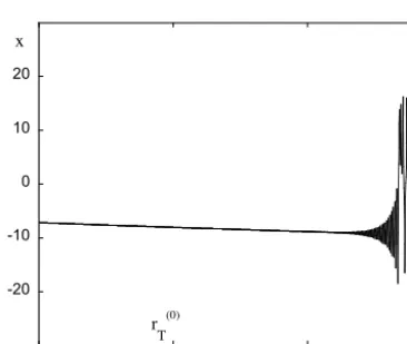
Figure 5, to be compared with Fig. 1, depicts the evolution of variablex versus time (expressed in terms of parameter
r=r0+t) as obtained from direct numerical integration of Eqs. (13) and (14) forr0=20 and=0.01. Once again the system runs across the static transition pointrT(0)≈24.74, re-mains close to the reference state (x−,y−,z) and eventually
evolves toward a chaotic state at a time corresponding to a valuercbetween 29 and 30, in excellent agreement with the theoretical predictions summarized in Fig. 4. This result re-mains robust in the sense thatrcis essentially determined by
r0independent offor a wide range ofvalues. But asis increased one witnesses deviations from the theoretical esti-mate as illustrated in Fig. 6, where for the same value ofr0 as before and for=0.1 the transition to the chaotic regime occurs at a value ofrof about 32.
-20 -10 0 10 20
20 25 30 r
x
r
T (0)
Figure 5. Time evolution of variable x of model (13) expressed
in terms of the instantaneous value ofr with=0.01 and initial conditionx=x−,y=y−,z=r0−1.
-20 -10 0 10 20
20 25 30 r
x
r T
(0)
Figure 6.As in Fig. 5 but with=0.1.
level higher than its value in the reference state. Figure 7 summarizes the results obtained by numerically integrating Eqs. (13) and (14) for a wide range of values of and for a threshold value of |x/x±| =1.5. We observe an
increas-ing trend similar to the one reported in Fig. 3, reflectincreas-ing the enhancement of stabilization of the reference state upon increasing the rate at which the bifurcation diagram is tra-versed.
Assuming now that the system has settled in the chaotic regime, we wish to quantify in some way the effect of the time variation of parameterron the behavior of the principal variables involved. A first result in this direction is reported in Fig. 8a, where the instantaneous ensemble averages over 100 000 initial conditions lying on the initial attractor of x,
y andzare plotted against time as measured again byr=
r0+t for values between 26 and 36, for which the system shows chaotic behavior. We see thatxandyhardly perceive the time-dependent forcing, whereaszfollows it in a rather straightforward manner. This shows how subtle the response of system to a parameter may be. Notice, however, that a
30 35 40
0 0.2 0.4 0.6 0.8 1
r
Figure 7.As in Fig. 3 but for model (13) withr0=20 and threshold
value|x/x±| =1.5. Other parameter values as in Fig. 4.
further increase inrmay bring the system to a new attractor and change the qualitative features of the dynamics.
Figure 8b depicts the time evolution (again via the de-pendence onr(t )) of the variances ofx,y andz variables around their means. We see that they all follow a systematic increasing trend. This suggests the possibility that variance can serve as a key quantity and as an early warning of future changes induced by a time-dependent forcing, especially as far as the occurrence of extreme events is concerned (Chavez et al., 2016).
5 Transitions between states and limit point bifurcations
There is ample evidence of large-scale climatic transitions between glacial and interglacial regimes (Berger, 1981). On a shorter timescale transitions between different global cir-culation patterns associated to the phenomenon of persistent flow regimes at mid-latitudes, also referred to as “blocking” in contrast to the familiar zonal flows, are well documented and constitute one of the principal elements of low-frequency atmospheric variability.
0 10 20 30
28 32 r 36
< x > < y >
< z >
(a)
60 80 100
28 32 r 36
< x2>
< y2
> < z2>
(b)
Figure 8.Ensemble averages(a)and variances(b)of variablesx,y, andzof model (13) in the chaotic regime versus the instantaneous value
of the ramp parameterrstarting fromr0=26 with=0.01. The number of initial conditions is 100 000.
0.1 1
0 2 4 6
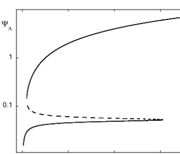
Figure 9.Bifurcation diagram of model (17) as parameterψA∗
in-creases from 0.05 to 7. Full lines represent the two stable solu-tions, blocked (lower), zonal (upper) and dashed line the inter-mediate unstable state. Parameter valuesk=10−2,β=0.1,h1=
1.6
√
2/(3π ),h2=h1/5 andα=8h1.
dψA
dt = −k ψA−ψ ∗ A
+h1ψL,
dψK
dt = −(αψA−β) ψL−kψK,
dψL
dt =(αψA−β) ψK−h2ψA−kψL. (17)
HereψA,ψK, andψLdenote the amplitudes of the three
retained modes,ψA∗is a forcing parameter of the flow andk
accounts for the effect of the dissipation. The remaining pa-rameters are related to the topography and to the mean height of the fluid layer. Higher-order truncation schemes have been developed by Ghil and coworkers (Legras and Ghil, 1985).
Figure 9 depicts the bifurcation diagram of model (17) in which the zonally averaged velocity mode ψA is plotted
against the forcing parameterψA∗, keeping the other parame-ters fixed (see caption). One observes two branches of stable solutions (full lines) colliding and terminating with an
in-termediate unstable branch (dashed line) at two critical val-ues corresponding to a limit point bifurcation. Going back to the space dependence of the velocity field, one finds that the lower branch corresponds to the state of atmospheric block-ing, whereas the upper branch is representative of zonal flow (Charney and De Vore, 1979; Egger, 1981; Nicolis, 2002).
In what follows we chooseψA∗ as the forcing parameter, setting
ψA∗=ψ0∗+t. (18)
Figure 10 summarizes the results of numerical simulations of the full Eqs. (17) and (18) for three different initial con-ditions that in the absence of time variation ofψA∗ would all be attracted by the lower (stable) branch of solutions. We see that in actual fact this branch is skipped altogether and the trajectories evolve to the upper stable branch passing through the intermediate unstable one. Interestingly, they are all significantly delayed before reaching eventually the up-per branch. Part of this delay can be attributed to the slowing down of the dynamics in the vicinity of the limit point, where the generalized eigenvalues of the Jacobian around the upper branch tend to zero forψA∗ tending to its value at the limit point.
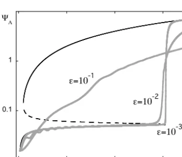
A second series of numerical simulations is reported in Fig. 11, starting this time from a state in the vicinity of the lower stable branch. For very smallwe see that the branch is followed up to the rightmost point, whereupon the trajec-tory jumps to the upper branch with practically no delay. But asis increased, one witnesses increasingly early departures from the reference state. The corresponding trajectories pass through the intermediate unstable branch and tend to the up-per one, reaching it with delays that increase markedly with
tem-0.1 1
0 1 2
(a)
(b)
(c)
Figure 10.Time evolution of variableψAof model (17) in the
pres-ence of a time-dependent forcing (Eq. 18). Initial conditions(a),(b) and(c)evolve to the zonal state (upper stable branch of the bifurca-tion diagram), although in the absence of the time-dependent forc-ing the system is bound to follow the blocked circulation solution (low stable branch of the bifurcation diagram). Parameter values
=0.01 and as in Fig. 9.
0.1 1
0 2 4 6
=10-3
=10-2
=10-1
Figure 11.As in Fig. 10 but for initial conditions in the vicinity of
the lower stable branch of the bifurcation diagram and three differ-entvalues.
porarily pass a threshold beyond which it starts being at-tracted by the upper branch.
A more quantitative explanation, albeit limited to the vicinity of the limit points, appeals to the fundamental result that in the vicinity of a limit point bifurcation the dynam-ics simplifies considerably. Specifically, there exists a single variablezrelated to combinations of the three original vari-ables appearing in Eq. (17), to which one refers as the order parameter, satisfying a universal equation of the form (Guck-enheimer and Holmes, 1983)
dz
dt =µ(t )−z
2, (19)
whereµis a combination ofψA∗ and of the other parameters appearing in Eqs. (17) and (18).
Setting againµ(t )=µ0+t, one can show that upon ap-propriate scaling of variables and parameters Eq. (19) can be transformed to an Airy equation (Davies and Krishna, 1996). The solution in terms of the original variablezis then
z=1/3
Ai0µ0+t 2/3
+CBi0µ0+t 2/3
Aiµ0+t 2/3
+CBiµ0+t 2/3
. (20)
Here Ai and Bi are the Airy functions, the prime denotes the derivative with respect to the whole argument andC is determined by the initial conditionz(0)=z0. Carrying out at the level of Eq. (19) the numerical experiments summa-rized in Fig. 10, one can now delimit the initial conditions that will evolve to the upper stable branchz=õ(t )of the quasi-static solution of Eq. (19), by requiring that the denom-inator in Eq. (20) remains different from zero, which in turn requires thatCbe positive. This yields trajectories behaving for the original dynamical system according to Fig. 10 (Nico-lis and Nico(Nico-lis, 2014). Notice that the approach outlined in Sect. 2 and applied successfully in Sects. 3 and 4 is not ap-propriate in the presence of a limit point, since the reference stable state does not continue beyond the bifurcation point as an unstable branch of solutions, but disappears altogether.
6 Conclusions
In this work we identified some universal trends underlying the response of a system to systematic changes of parame-ters in time. Most prominent among them are that, starting with a stable branch of states, transitions to new regimes that would occur in the “static” case of absence of time variation of parameters tend to be delayed; states that in the static case are unstable are temporarily stabilized; and states that in the static case are stable can be skipped altogether. As a corol-lary, the times at which threshold values are first crossed have been obtained as a function of the rate of increase of the pa-rameters in time.
These conclusions were based on a generalized stability criterion extending classical stability analysis to account for the presence of time-varying coefficients in the evolution equations of the system’s variables, as well as on analytic solutions prevailing in the vicinity of transition points. They were validated by the results of numerical integration of the evolution equations of prototypical systems of relevance in atmospheric and climate dynamics giving rise to periodic be-havior, to chaotic dynamics and to transitions between si-multaneously stable steady states. As it turned out for suf-ficiently small rates of parameter change a universal, -independent regime is reached in which the transition occurs at a parameter value depending entirely on the initial value and the critical value corresponding to the limit=0. But as
The extended stability analysis followed in this work be-longs to the class of linear response theories, in the sense that it is focussing on the conditions under which perturba-tions, initially assumed to be small, will at some stage start to grow in time. On the other hand it is purely deterministic, as random external perturbations or intrinsic fluctuations have not been incorporated into the description. A different class of linear response theories was recently developed in the cli-mate literature (see, e.g., Lucarini, 2012; Nicolis and Nicolis, 2015) in which the change in the fluctuation properties of a system due to the presence of noise and the response of the noise-free system to deterministic forcings were linked. Im-plicit in these approaches is the existence of a well-defined invariant probability measure of the reference system with re-spect to which statistical averages are carried out. Our anal-ysis suggests that this can be so under the conditions that the system is operating around a well-defined, single stable regime, i.e., (a), that the range of variations of the forcing is nested between two successive bifurcation points; and (b), that the rateis sufficiently small so that the instantaneous perturbation to the invariant probability brought by the forc-ing remains small.
Throughout our approach the time variation of the param-eters has been fully and consistently incorporated into the intrinsic time evolution of the system’s variables as given by the appropriate rate equations. Our results depend critically on this view of parameter-system co-evolution, a scenario reflecting, we believe, the way a natural system is actually evolving in time. This scenario differs from those adopted in current studies on climatic change based on the integration of large numerical models, where parameters are suddenly set at a different level and the system is subsequently left to relax under these new conditions. It would be interesting to allow for different scenarios beyond the standard ones, closer to our fully dynamical approach, and to test the robustness of the conclusions reached under these different conditions.
Data availability. Data can be accessed by directly contacting the author. They are not publicly accessible because they have been cre-ated for the specific purposes of the present work.
Competing interests. The authors declare that they have no conflict of interest.
Special issue statement. This article is part of the special issue “Numerical modeling, predictability and data assimilation in weather, ocean and climate: A special issue honoring the legacy of Anna Trevisan (1946–2016)”. It is not associated with a conference.
Edited by: Juan Manuel Lopez Reviewed by: two anonymous referees
References
Andrews, T., Gregory, J. M., Webb, M. J., and Taylor, K. E.: Forcing, feedbacks and climate sensitivity in CMIP5 coupled atmosphere-ocean climate models, Geophys. Res. Lett., 39, LO9712, https://doi.org/10.1029/2012GL051607, 2012. Ashwin, P., Wieczorek, S., Vitolo, R., and Cox, P.: Tipping points in
open systems:Bifurcation noise-induced and rate-dependent ex-amples in the climate system, Phil. Trans. R. Soc. A, 370, 1166– 1184, 2012.
Baer, S. M., Erneux, T., and Rinzel, J.: The slow passage through a Hopf bifurcation: delay, memory effects, and resonance, SIAM J. Appl. Math., 49, 55–71, 1989.
Benoit, E.: Dynamic Bifurcations, Springer, Berlin, 222 pp., 1991. Berger, A.: Climatic Variations and Variability: Facts and Theories,
Reidel, Dordrecht, 795 pp., 1981.
Charney, J. and De Vore, J.: Multiple flow equilibria in the atmo-sphere and blocking, J. Atmos. Sci., 36, 1205–1216, 1979. Chavez, M., Ghil, M., and Urrutia-Fucugauchi, J.: Extreme Events:
Observations, Modeling, and Economics, Geophysical Mono-graph Series vol. 214, Wiley, Hoboken, 423 pp., 2016.
Davies, H. G. and Krishna, R.: Nonstationary response near generic bifurcations, Nonl. Dyn., 10, 235–250, 1996.
Dijkstra, H. A.: Nonlinear Climate Dynamics, Cambridge Univer-sity Press, Cambridge, 367 pp., 2013.
Erneux, T. and Mandel, P.: Imperfect bifurcation with a slowly-varying control parameter, SIAM J. Appl. Math., 46, 1–15, 1986. Egger, J.: Stochastically driven large-scale circulations with
multi-ple equilibria, J. Atmos. Sci., 38, 2608–2618, 1981.
Essex, C. and McKitrick, R.: Taken by Storm, Key Porter Books, Toronto, 365 pp., 2007.
Goodie, A. S. and Guff, D.: Encyclopedia of Global Change, Oxford University Press, Oxford, 1424 pp., 2001.
Gregory, J. M., Andrews, T., and Good, P.: The incon-stancy of the transient climatic response parameter un-der increasing CO2, Phil. Trans. R. Soc., 373, 20140417, https://doi.org/10.1098/rsta.2014.0417, 2015.
Guckenheimer, J. and Holmes, P.: Nonlinear Oscillations, Dynam-ical Systems and Bifurcations of Vector Fields, Springer, New York, 459 pp., 1983.
Kevorkian, J. K. and Cole, J. D.: Multiple Scale and Singular Per-turbation Methods, Springer, New York, 634 pp., 1996. Legras, B. and Ghil, M.: Persistent anomalies, blocking and
varia-tions in atmospheric predictability, J. Atmos. Sci., 42, 433–471, 1985.
Lorenz, E. N.: Deterministic non-periodic flow, J. Atmos. Sci., 20, 130–141, 1963.
Lorenz, E. N.: Irregularity, a fundamental property of the atmo-sphere, Tellus A, 36, 98–110, 1984.
Lucarini, V.: Stochastic perturbations to dynamical systems: A re-sponse theory approach, J. Stat. Phys., 146, 774–786, 2012. Nicolis, C.: Self-oscillations and predictability in climate dynamics,
Tellus A, 36, 1–10, 1984.
Nicolis, C.: Transient climatic response to increasing CO2
concen-tration: some dynamical scenarios, Tellus A, 40, 50–60, 1988. Nicolis, C.: Irreversible thermodynamics of a simple atmospheric
Nicolis, C. and Nicolis, G.: Noisy limit point bifurcation with a slowly varying control parameter, Europhys. Lett., 66, 185–191, 2004.
Nicolis, C. and Nicolis, G.: Dynamical responses to time-dependent control parameters in the presence of noise:
a normal form approach, Phys. Rev., E89, 022903,
https://doi.org/10.1103/PhysRevE.89.022903, 2014.
Nicolis, C. and Nicolis, G.: The fluctuation-dissipation theorem re-visited: Beyond the Gaussian approximation, J. Atmos. Sci., 72, 2642–2656, 2015.
Saltzman, B., Sutera, A., and Hansen, A. R.: A possible marine mechanism for internally-generated long-period climatic cycles, J. Atmos. Sci., 39, 2634–2637, 1982.
Sparrow, C.: The Lorenz Equations, Springer, New York, 269 pp., 1982.