Compacting the description of a time-dependent multivariable system and its multivariable driver by reducing the state vectors to aggregate scalars: the Earth's solar-wind-driven magnetosphere

https://doi.org/10.5194/npg-26-429-2019 © Author(s) 2019. This work is distributed under the Creative Commons Attribution 4.0 License.

Compacting the description of a time-dependent multivariable

system and its multivariable driver by reducing the state vectors to

aggregate scalars: the Earth’s solar-wind-driven magnetosphere

Joseph E. Borovsky1and Adnane Osmane2

1_{Center for Space Plasma Physics, Space Science Institute, Boulder, Colorado, USA} 2_{Department of Physics, University of Helsinki, Helsinki, Finland}

Correspondence:Joseph E. Borovsky ([email protected]) Received: 21 January 2019 – Discussion started: 20 May 2019

Revised: 20 May 2019 – Accepted: 22 August 2019 – Published: 22 November 2019

Abstract. Using the solar-wind-driven magnetosphere– ionosphere–thermosphere system, a methodology is devel-oped to reduce a state-vector description of a time-dependent driven system to a composite scalar picture of the activity in the system. The technique uses canonical correlation analysis to reduce the time-dependent system and driver state vectors to time-dependent system and driver scalars, with the scalars describing the response in the system that is most-closely re-lated to the driver. This reduced description has advantages: low noise, high prediction efficiency, linearity in the de-scribed system response to the driver, and compactness. The methodology identifies independent modes of reaction of a system to its driver. The analysis of the magnetospheric sys-tem is demonstrated. Using autocorrelation analysis, Jensen– Shannon complexity analysis, and permutation-entropy anal-ysis the properties of the derived aggregate scalars are as-sessed and a new mode of reaction of the magnetosphere to the solar wind is found. This state-vector-reduction technique may be useful for other multivariable systems driven by mul-tiple inputs.

1 Introduction

In this report a methodology is described that can produce a compact description of the behavior of a time-dependent, multivariable system driven by a time-dependent, multivari-able driver or by multiple drivers. The system used to develop this methodology is the Earth’s magnetosphere–ionosphere– thermosphere system driven by the time-dependent solar

wind. The spatial domain wherein the Earth’s magnetic field dominates over the solar wind is known as the magneto-sphere. The interaction between the solar wind, and the mag-netosphere is surprisingly complex and the magmag-netosphere’s evolution in response to the time-varying solar wind is rich and diverse. The magnetospheric system is characterized by multiple subsystems that interact with each other (cf. Lyon, 2000; Otto, 2005; Siscoe, 2011; Eastwood et al., 2015; Borovsky and Valdivia, 2018): almost 6 orders of magnitude of spatial scales are involved in the global behavior of the magnetosphere, from ∼1 to∼6×105km. This system is highly coupled, dynamic, with memory and with feedback loops. Multiple physical processes act to couple the various subsystems, with the strength of the couplings evolving with time as the subsystems evolve owing to the couplings. Even after a half of a century of measurements and analysis, its subsystems and the couplings between its subsystems are not fully understood (Stern, 1989, 1996; Denton et al., 2016). It has been argued that the system adjectives “adaptive”, “non-linear”, “dissipative”, and “complex” apply to the magneto-spheric system (Borovsky and Valdivia, 2018). (See also the earlier systems analyses by Horton et al., 1999, Chapman et al., 2004, Valdivia et al., 2005, 2013, and Sharma, 2010.) The magnetospheric system is well measured: there are hundreds of thousands of hours of simultaneous measurements of var-ious aspects of the magnetospheric system and its solar-wind driver over the five decades of the “space age” (cf. Stern, 1989, 1996; King and Papitashvili, 2005).

vari-ables describing the system may be intercorrelated, and the variables describing the driving may be intercorrelated. The methodology was developed to gain an understanding of the Earth’s magnetosphere–ionosphere–thermosphere sys-tem as driven by the solar wind. To utilize the methodol-ogy the system and its driver are conceptualized by a time-dependent, multidimensional system state vectorS(t )and a time-dependent, multidimensional driver state vector D(t ), with the assumption that the driver vectorDaffects the sys-tem vectorS, but not vice versa, writtenD→S. The individ-ual time-dependent scalar variables making up the state vec-torS(t )are time-dependent measures of various forms of ac-tivity in the system and various properties of the system, and the individual time-dependent scalar variables making up the driver state vectorD(t )are various time-dependent measures of the properties of the drivers of the system. We will utilize the correlation properties between the components (individ-ual time-dependent variables) ofSand the components ofD. Canonical correlation analysis (CCA) will be used to derive scalar projections (dot products) of S(t )and scalar projec-tions of D(t ) that have the highest Pearson linear correla-tion coefficient between them. The derived scalar projeccorrela-tions S(1)(t ),S(2)(t ),S(3)(t ), . . .of the vectorS(t )will be

com-posite (aggregate) measures of activity in the system, and the derived scalar projectionsD(1)(t ),D(2)(t ),D(3)(t ),. . .of the

vectorD(t )will be the composite drivers ofS(1)(t ),S(2)(t ),

S(3)(t ),. . ., respectively. In essence, the aggregate variables

S(1)(t ),S(2)(t ),S(3)(t ),. . .are “latent variables” of the

sys-tem constructed from the “manifest variables” in the syssys-tem state vector. This reduced scalar picture D(i)→S(i) of the

system driven by the driver focuses on the time-dependent properties of the system that react to the driver. By maxi-mizing the correlations, the predictability of the system from knowledge of the state of the driver is also maximized.

The solar-wind-driven magnetospheric system very cleanly follows theD→Spicture where the driver affects the system, but the system does not affect the driver. The Earth’s magnetosphere has no influence whatsoever on the properties of the solar wind that passes the Earth. Measurements of this magnetospheric system will be used in Sects. 2 and 3 to explore the mathematical reduction of the state-vector D(t )→S(t ) picture to the composite-scalar D(i)(t )→S(i)(t ) picture. Table 1 lists the nine

time-dependent measurements of the magnetosphere in the system state vector S and the eight time-dependent measurements of the solar wind in the driver state vectorD. The individual variables in the system state vector and in the driver state vector are described in the Appendix.

This report is organized as follows. In Sect. 2 the CCA approach is applied to the magnetospheric system driven by the solar wind to derive the first three time-dependent sets of composite variablesS(1)(t )andD(1)(t ),S(2)(t )and

D(2)(t ), andS(3)(t )andD(3)(t )from the state vectorsS(t )

and D(t ). In Sect. 3 the three sets of composite variables S(i) andD(i) for the magnetospheric system are explored,

and the complexity–entropy properties of the aggregate vari-ableS(1)(t )are analyzed. In Sect. 4 the advantages of the

re-ducedD(i)→S(i)scalar description are examined: these

ad-vantages include (a) a compact description of global system-wide reactions to variations in the driver, (b) increased pre-dictability of the system from knowledge of the driver, (c) linearity in the description of the system’s response to the driver, and (d) lower noise in correlations between the system variables and the driver variables. The reduced scalar picture can also reveal independent modes of reaction of the system to the driver, providing insight into the behavior of the system in reaction to complexities in the driver. The vari-ables of the magnetospheric and solar-wind state vectors are described in the Appendix.

2 Creation of composite (aggregate) variables from the state vectors

Using the Earth’s magnetosphere–ionosphere–thermosphere system as driven by the solar wind, the reduction of a time-dependent state-vector pictureD(t )→S(t )to the time-dependent composite-variable-pair pictureD(i)(t )→S(i)(t )

will be performed. The nine measured variables chosen for the nine-dimensional magnetospheric system state vectorS

appear in the first column of Table 1, and the eight measured variables chosen for the eight-dimensional solar-wind driver state vectorDappear in the second column of Table 1, with explanations of those measures deferred to the Appendix.

One-hour averages of all magnetospheric and solar-wind variables are used in the years 1991–2007. No time lags are used between the solar-wind measurements and the magneto-spheric measurements: most expected time lags will be about 1 h (e.g., Clauer et al., 1981; Smith et al., 1999), which is the time resolution of the data set.

Canonical correlation analysis (CCA) is applied to the time-dependent state vectorsS(t )andD(t ). CCA finds cor-relation patterns between two multivariable data sets (Nimon et al., 2010; Hair et al., 2010). It yields pairs of compos-ite (aggregate) variables (a) that are linear combinations of the variables of the two data sets and (b) that have maximal correlations with each other. Each pair of composite vari-ables is called the “Nth canonical correlation”. From the data sets ofS(t ) andD(t )the first pair of composite variables yielded (the first canonical variates) isS(1)(t )andD(1)(t ):

these two variables are projections of S and D given by S(1)(t )=CS1·S(t )andD(1)(t )=CD1·D(t ), whereCS1and

CD1are time-independent coefficient (weight) vectors.S(1)

andD(1)are the composite variables fromSandDthat have

the highest Pearson linear correlation coefficient with each other. Here, CCA is in a sense creating the system func-tion S(1)(t )that is most reactive to the driver vector D(t )

and creating the driver scalar functionD(1)(t )that describes

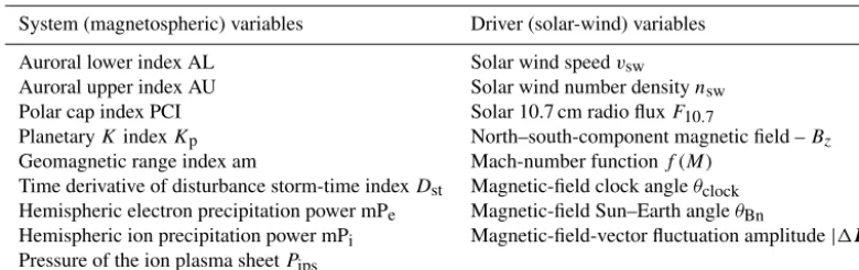
Table 1.The nine time-dependent variables going into the system state vectorS(t )of the magnetosphere and the eight time-dependent variables going into the driver state vectorD(t )of the solar wind.

System (magnetospheric) variables Driver (solar-wind) variables

Auroral lower index AL Solar wind speedvsw

Auroral upper index AU Solar wind number densitynsw Polar cap index PCI Solar 10.7 cm radio fluxF10.7

PlanetaryKindexKp North–south-component magnetic field –Bz

Geomagnetic range index am Mach-number functionf (M) Time derivative of disturbance storm-time indexDst Magnetic-field clock angleθclock Hemispheric electron precipitation power mPe Magnetic-field Sun–Earth angleθBn

Hemispheric ion precipitation power mPi Magnetic-field-vector fluctuation amplitude|1B| Pressure of the ion plasma sheetPips

andD(3)(the third canonical correlation), etc.S(2)andD(2)

are the projections of SandD that have the highest corre-lation with each other, provided thatS(2) andD(2) are

un-correlated with S(1) andD(1).S(3) andD(3) are the

projec-tions ofSandDthat have the highest correlations with each other, provided they are uncorrelated with S(1), S(2),D(1),

and D(2).S(1)(t ),S(2)(t ), and S(3)(t )represent three

inde-pendent modes of reaction of the global system to the driver

D(t ). The CCA process will identify these modes (and their respective drivers).

CCA is a matrix equation solution, non-iterative, that yields a single unique solution (Johnson and Wichern, 2007). CCA operates on standardized variables (with the mean value subtracted and the values then divided by the standard deviation), denoted with an asterisk. (For each variable the mean value and standard deviation are calculated for the en-tire data set.) CCA operates most efficiently on variables that are Gaussian distributed: hence the logarithms of some vari-ables are used to yield more-Gaussian-like distributions. All standardized variablesv∗have a mean value of zero, a stan-dard deviation unity, and no units.

When CCA is applied to the 1991–2007 S(t )andD(t ) data sets (see Table 1), the first canonical pair of time-dependent variables is

S(1)=0.0260log10(1+ |AL|)

∗

+0.1151log₁₀(1+ |AU|)∗+0.2160|PCI|∗ +0.1451Kp∗+0.2881log10(1+am)

∗

+0.0201d|Dst|/dt∗+0.0492log₁₀(0.01+mPe)∗

+0.2531log₁₀(0.01+mPi)∗

+0.0854log₁₀ 0.01+Pips

∗

(1a) D(1)=0.8378log10(vsw)

∗₊

0.6876log₁₀(nsw)∗

+0.1018log₁₀(F10.7)∗−0.1676(−Bz)∗

+0.3547f (M)∗+0.3844Dsin2(θclock/2)

E∗

3

+0.0960hθBni∗3+0.0943log10(0.1+ |1B|)

∗

. (1b)

S(1)andD(1)have mean values of zero and standard

devia-tions of unity. The derived composite variables given by ex-pressions (1) are robust and reproducible: applying the CCA process to various subsets of the full 1991–2007 data set, the CCA process repeatedly yields essentially the same coeffi-cients that are in Eqs. (1a) and (1b) (cf. Borovsky and Den-ton, 2018).

CCA applied to the time-dependent state vectorsS(t )and

D(t )for the 1991–2007 data set yields the second canonical pair of time-dependent scalar variables as

S(2)= −0.2628log10(1+ |AL|)

∗

−0.0874log₁₀(1+ |AU|)∗−0.1302|PCI|∗ −0.0556Kp∗+0.1928log10(1+am)

∗

+0.0028d|Dst|/dt∗−0.8506log₁₀(0.01+mPe)∗

+0.9218log₁₀(0.01+mPi)∗

+0.3493log₁₀ 0.01+Pips

∗

(2a) D(2)=0.1195log10(vsw)

∗₊

0.8874log₁₀(nsw)∗

+0.1202log₁₀(F10.7)∗−0.1138(−Bz)∗

+0.2669f (M)∗−0.5079Dsin2(θclock/2)

E

3

∗

−0.0186hθBni∗3+0.0260log10(0.1+ |1B|)

∗

. (2b) For the 1991–2007 data set CCA yields the third canonical pair of time-dependent scalar variables as

S(3)= −0.1796log10(1+ |AL|)

∗

−0.2220log₁₀(1+ |AU|)∗−1.0351|PCI|∗ +0.8265Kp∗+0.5809log10(1+am)

∗

−0.2169d|Dst|/dt∗+0.3856log₁₀(0.01+mPe)∗

−0.6100log₁₀(0.01+mPi)∗

+0.1064log₁₀ 0.01+Pips

∗

(3a) D(3)=0.4241log10(vsw)

∗₋

0.1985log₁₀(nsw)∗

−0.1404log₁₀(F10.7)∗−0.6704(−Bz)∗

−0.1008f (M)∗+0.0572Dsin2(θclock/2)

E∗

3

−0.3134hθBni∗3+0.3055log10(0.1+ |1B|)

∗

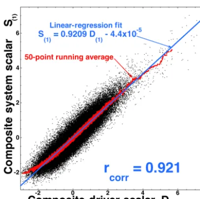
Figure 1.The aggregate system scalarS(1)is plotted as a function

of the driver scalarD(1)for the 1 h resolution 1991–2007 data set.

Each black point is 1 h of data.

The properties ofS(1)(t )andD(1)(t ),S(2)(t )andD(2)(t ), and

S(3)(t )andD(3)(t )as given by Eqs. (1)–(3) are explored in

Sect. 3.

3 Properties of the scalar reduced picture for the magnetospheric system

The three sets of composite variablesS(1)andD(1),S(2)and

D(2), andS(3)andD(3)for the magnetospheric system are

ex-plored and the advantages of the reducedD(i)→S(i)scalar

description are investigated.

3.1 The primary mode of system response as represented byD(1)→S(1)

In Fig. 1 the composite system variable S(1) (as given by

Eq. 1a) is plotted for the years 1991–2007 as a function of the composite driver variableD(1)(as given by Eq. 1b). Each

black point in Fig. 1 represents 1 h of data. The Pearson linear correlation coefficient between S(1) andD(1) for the 1991–

2007 data set isrcorr=0.921. Accordingly,r_corr2 =84.8 % of the variance of the system function S(1)(t )is described by

the driver functionD(1)(t ), and so 15.2 % of the variance of

S(1) is unaccounted for by D(1). The blue line in Fig. 1 is

a linear-regression fit toS(1), and the red curve is a 50-point

vertical running average of the black points. Note the approx-imate linearity of system variableS(1)as a function of driver

variableD(1), indicated by the manner in which the running

average tracks the linear-regression line.

Note that whereas the correlation coefficient between S(1)(t )andD(1)(t )isrcorr=0.921, the maximum correlation coefficient between any single variable in the system state

vectorS(t )and any single variable in the driver state vec-torD(t )is onlyrcorr=0.586 (between

sin2(θclock/2)

3and log₁₀(1+ |AL|)).

As a further note, the Pearson linear correlation coeffi-cients betweenS(1)and various “physics-based” solar-wind

driver functions from the literature are the following:+0.378 for −vswBz, +0.557 for vswBsouth (Eq. 2 of Holzer and Slavin, 1979),+0.679 for the Newell function d8/dt(Eq. 1 of Newell et al., 2007),+0.723 for the quick reconnection functionRq(Eq. 8 of Borovsky and Birn, 2014), and+0.761 for the nonlinear reconnection-coupled MHD generator with Bohm viscosity (Eq. 65 of Borovsky, 2013). All of these driver functions have poor correlations withS(1)in

compari-son with the+0.921 correlation ofD(1)withS(1).

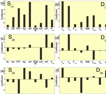
In the six panels of Fig. 2 the coefficients of the six vec-torsCS1,CD1,CS2,CD2,CS3, andCD3are plotted. (These are the coefficients in Eqs. 1–3.) Examining these six pan-els enables the reaction modes represented byS(1),S(2), and

S(3)to be interpreted as well as their driversD(1),D(2), and

D(3). Figure 2a indicates that all coefficients ofS(1)are

pos-itive: this indicates a mode of the magnetospheric system in which all measures of activity in the system vectorSincrease or decrease in unison, withS(1) representing a “global

ac-tivity index”. Figure 2b indicates that all of the coefficients ofD(1)are positive. The variables in the driver state vector

D (Table 1) and their signs were all chosen so that a pos-itive increase in each variable would result in a generally accepted increase in magnetospheric activity. The individual variables on the right-hand side of Eq. (1b) have all been cor-relatively associated with the driving of magnetospheric ac-tivity (Berthelier, 1976; Borovsky and Funsten, 2003; Newell et al., 2007; Borovsky and Denton, 2014; Borovsky and Birn, 2014; Osmane et al., 2015).S(1)is selected by the CCA

pro-cess to have highest correlation with solar-wind variability: S(1)is focused on activity that reacts to the solar-wind driver.

Using the linear-regression curve in Fig. 1 as a “predic-tion” of the value of S(1) from knowledge of the value of

D(1)yields

S(1)pred=0.9209D(1)−4.4×10−5. (4)

In Fig. 3 the autocorrelation functions ofS(1)(t )(red curve),

D(1)(t )(blue curve), andS(1)(t )−S(1)pred(t )(green curve) are plotted. In Fig. 3a it is seen that the autocorrelation func-tions ofS(1)andD(1)are very similar, with 1/e

autocorrela-tion times of 23.3 h forS(1)and 22.7 h forD(1). In Fig. 3b the

three autocorrelation functions are plotted for time shifts up to 40 d. Note the 27 d peak in the autocorrelation functions ofD(1)(t )andS(1)(t ): this is associated with the 27 d

rota-tion period of the Sun as viewed from the Earth and the per-sistence of features on the solar surface that give rise to so-lar wind with characteristic properties. This causes the driver

D(t )properties to have a 27 d periodicity, which drives the systemS(t )with a 27 d periodicity.

The quantityS(1)−S(1)predis the portion ofS(1)(t )that is

vari-Figure 2.Plots of the nine components of the coefficient vectors used to project the system state vectorSinto the aggregate variablesS(1)(a),

S(2)(c), andS(3)(e)and plots of the eight components of the coefficient vectors used to project the driver state vectorDinto the driver scalar

variablesD(1)(b),D(2)(d), andD(3)(f).

ance of S(1)(t ).S(1)(t )−S(1)pred(t )is completely uncorre-lated withD(1)(t ). Further,S(1)(t )−S(1)pred(t )is completely uncorrelated with each of the eight individual solar-wind variables on the right-hand side of Eq. (1b). Since S(1) is

so similar toD(1), the standard analyses of theS(1)(t )time

series (e.g., determining the correlation dimension, exam-ining the state space, or Fourier analyzing; Sharma et al., 2005a; Vassiliadis, 2006) would largely be an analysis of the properties of the solar-wind time seriesD(1)(t )– not so

forS(1)(t )−S(1)pred(t ), which is uncorrelated withD(1). The

autocorrelation function of S(1)(t )−S(1)pred(t )in Fig. 3a is

very different from the autocorrelation function ofD(1): the

1/eautocorrelation time ofS(1)(t )−S(1)pred(t )is 2.4 h.

De-termining what the unaccounted-for varianceS(1)−S(1)pred originates from is of great interest. Four suggestions of what contributes toS(1)−S(1)predare made here. First, some frac-tion ofS(1)−S(1)predmay be associated with noise in the var-ious measurements of the magnetospheric system and of the solar wind. Shot noise (random noise in the values of the vari-ables) would have an autocorrelation time of less than 1 h, the autocorrelation function of the shot-noise going from 1 to 0 in one data-resolution time shift (cf. Sect. 2.4 of Borovsky et al., 1997). Second, some fraction ofS(1)(t )−S(1)pred(t )may

be owed to errors in the measurement values in the state vec-torsS(t )andD(t ). Errors in the values of the variables ofD

could be caused by the spatial structure of the solar wind and the measuring spacecraft upstream of the Earth not intercept-ing the exact solar-wind structures that hit and drive the Earth (cf. Weimer et al., 2003; Borovsky, 2018a): this could affect all of the variables ofD. Extrapolating local measures to es-timate global properties can also lead to errors: this might af-fect the hemispheric particle-precipitation variables mPeand mPi(Emery et al., 2008) inS and also the magnetospheric pressure valuesPips(Borovsky, 2017) inS. Variables react-ing to more than one physical process (such as d|Dst|/dt and Pips)could also appear to have error in the values when re-lating the values toD(1). Third, unaccounted-for time lags

Figure 3.The autocorrelation functions for the system scalarS(1)

(red), the driver scalarD(1) (blue), and the unaccounted-for

vari-anceE(1)E(1)pred(green) are plotted. In panel(a)the plot extends to 50 h and in panel(b)the plot extends to 40 d.

time duration of a magnetospheric substorm (Borovsky et al., 1993; Weimer, 1994; Chu et al., 2015). Substorms are large transients in the reaction of the magnetospheric system to solar-wind driving. (Substorms have been described as self-organized criticality events in the driven magnetospheric sys-tem; Klimas et al., 2000.) The occurrence of a substorm is no-toriously difficult to predict from solar-wind data (Freeman and Morley, 2004; Hsu and McPherron, 2009; Newell and Liou, 2011). The timing of substorm occurrence would be particularly difficult to infer from the 1 h resolution variables going intoDbecause of the 3 h smoothing used on the clock-angle term

sin2(θclock/2)

3 in Eq. (1b) for D(1), with the clock angle being critical for substorm occurrence (Newell and Liou, 2011). The occurrence of a substorm would pro-duce signatures in many of the variables used inS(1),

typi-cally an enhancement in the variable’s amplitude lasting 2– 3 h (Weimer, 1994).

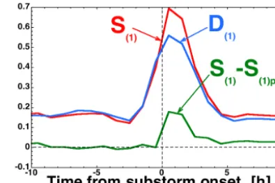
Figure 4.Superposed epoch averages ofS₍₁₎(red),D₍₁₎(blue), and S(1)−S(1)pred(green) for 2155 substorms. The epoch time (t=0) is the time of onset of each substorm.

To investigate this substorm hypothesis for S(1)(t )−

S(1)pred(t ), the variables D(1)(t ), S(1)(t ), and S(1)(t )−

S(1)pred(t ) are superposed-epoch averaged in Fig. 4 for a collection of 2155 substorm events; the collection is from Borovsky and Yakymenko (2017). The zero epoch in Fig. 4 is the onset time of each of the 2155 substorms. Substorms are associated with intervals of driving of the magnetosphere (e.g., Caan et al., 1977; Morley and Freeman, 2007); this is indicated by the increase in the superposed average ofD(1)

beginning prior to the onset time in Fig. 4. However, sub-storms also represent a transient release of stored energy in the magnetosphere (Birn et al., 2006); this is indicated in Fig. 4 by the superposed average ofS(1) exceeding the

su-perposed average ofD(1)after the substorm onset and by the

positive perturbation of theS(1)−S(1)predcurve after onset. TheS(1)−S(1)predcurve indicates a transient inS(1) that is

unaccounted for byD(1) associated with the occurrence of

substorms. The autocorrelation time of the green superposed-averageS(1)−S(1)pred time series plotted in Fig. 4 is 2.6 h, similar to the Fig. 1 autocorrelation time of the full 1991– 2007 time series ofS(1)−S(1)pred.

Compacting the description of the system from a multidi-mensional state vector to a few variablesS(1),S(2),S(3),. . .

is a form of dimensional reduction to a small set of funda-mental latent variables: in that dimensional reduction a po-tential question is whether the reduced (more-fundamental) variables themselves exhibit a reduction of their embedding dimension from the embedding dimensions of the manifest variables in the state vector. Additionally, it would be valu-able to differentiateS(1) from other indices commonly used

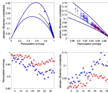
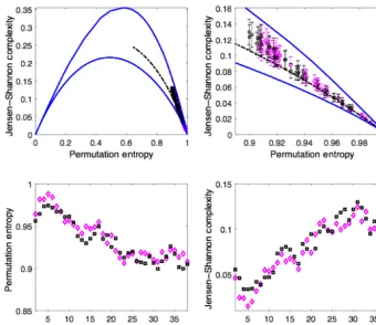
se-ries. In other words, one can seek timescales upon which co-herent structures/fluctuations/modes arise. In some instances, coherent modes are signatures of deterministic chaos (Maggs and Morales, 2013) or a reduction to the number of degrees of freedom (Osmane et al., 2019). Readers with little famil-iarity with these two information theoretic measures can con-sult the reviews of Riedl et al. (2013) and Zanin et al. (2012) or the pedestrian methodology section found in Osmane et al. (2019). In Figs. 5 and 6, we map the values of AL (red), am (blue),S(1) (black) andD(1) (pink) on the complexity–

entropy plane for an interval of 500 h duration with no data gaps, embedding dimensions of d=4, and embedding de-layT ranging between 2 and 40 h. Because there are a total ofd! =24 ordinal patterns we are limited to embedding de-lays of the order of 2 d. For embedding dede-lays greater than T =48 h the number of segmentsN−(d−1)∗T becomes too small to ascertain the likelihood of forbidden ordinal pat-terns. Error bars for the Jensen–Shannon complexity, shown for the zoomed panels of the complexity–entropy planes, are computed as the square root of the number of ordinal pat-terns divided by the number of segments available. Hence, larger embedded dimensions d, require a larger number of segments N−(d−1)∗T to determine whether the Jensen– Shannon complexity lies significantly above the stochastic boundary (see below).

The bottom left panels in Figs. 5 and 6 show the value of the permutation entropy for AL, am,D(1)andS(1)as a

func-tion of embedding delay. Similarly, the bottom right panels show the value of the Jensen–Shannon complexity for AL, am, D(1) andS(1) as a function of embedding delay. What

we notice is that all four signals are highly stochastic since the normalized permutation entropy is very close to 1. How-ever, we see that the Jensen–Shannon complexity forS(1)is

of comparable magnitude as for am, and it is significantly larger than for AL. This is not a surprise because the con-struction ofS(1) was based on am, and the Jensen–Shannon

complexity indicates that the former preserved the correlated structures of the latter on timescales ranging between a few hours to a few days. The top left panel of Figs. 5 and 6 shows the complexity–entropy plane, and the top right panel is a zoom of the right corner where most of the data for AL, am, and S(1) lies. In both figures the blue line curves

rep-resent the maximum and minimum value of complexity for a fixed entropy value, and the dashed curve represents the complexity–entropy mapping of fractional Brownian motion (fBm) with Hurst exponent ranging between 0 and 1, which is a stochastic process that also contains correlated structures. The fBm curve is a boundary between deterministic (above) and stochastic (below) fluctuations. We note that AL is ef-fectively stochastic, whereas am andS(1)lie above the fBm

boundary for a few tens of hours. The explanation for this be-havior from am lies in its construction: it is repeated for 3 h at a time. Hence, ordinal patterns of sized=4 and embedding delays of a few hours will register the repetition as correlated

structures. SinceS(1) is constructed in part with am, it also

contains part of its correlated structure.

For longer embedding delays of the order of seasonal vari-ations ranging from 27 to 45 d (not shown), all four time se-ries overlap and are indistinguishable from stochastic fluc-tuations. In terms of complexity–entropy plane it translates into a permutation entropy of approximately 1 and a Jensen– Shannon complexity of almost 0. Hence, the system variable S(1), based on various magnetospheric indices, preserves the

stochastic and correlational structures of its individual com-ponents. The comparable values of the permutation entropy (and therefore Jensen–Shannon complexity) with the system variable with the indices for long times are not fortuitous. The permutation entropy is invariant under any monotonic transformations (for instance, if one scales the time series by a positive real number, or if one takes the logarithm). However, if one used a linear combination of non-monotonic functions, for instance trigonometric functions, then the per-mutation entropy would not be invariant. Since the Jensen– Shannon complexity is a function of the permutation en-tropy, it is also invariant under monotonic transformations. Additionally, if one takes an average around the mean of some time series over a time TAU, one will reduce the noise level for fluctuations with timescales less than TAU. Thus, the stochastic nature of the signal will be reduced, and the permutation entropy and Jensen–Shannon complexity would move up in the plane towards the chaotic and/or periodic re-gions. The equivalence mapping of the information theoretic measures for the system variables and geomagnetic indices is a consequence of the monotonic transformation linking the former to the latter and the absence of coarse-graining of the indices.

3.2 The secondary modes of reaction represented by

S(2)andS(3)

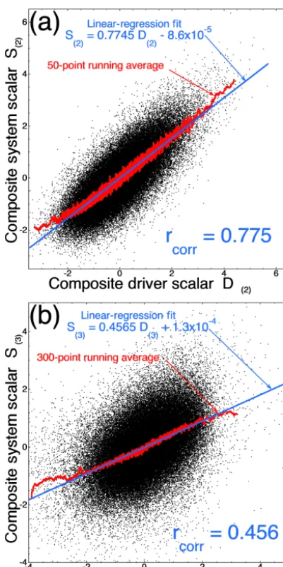
In Fig. 7a and b the second and third scalar pairs are plot-ted,S(2)as a function ofD(2)andS(3)as a function ofD(3),

respectively (Eqs. 2 and 3). The correlation coefficient for the second pair is still quite high (rcorr=0.775) but lower than that of the first pair (Fig. 1). This correlation coefficient rcorr=0.775 for the secondary mode is better than correla-tions obtained in most studies of solar-wind–magnetosphere coupling using single measures of the magnetospheric sys-tem (e.g., Table 3 of Newell et al., 2007; Table 1 of Borovsky, 2013).D(2)describesrcorr2 =60.0 % of the variance ofS(2).

In Fig. 7b the correlation coefficient for the third pair is low (rcorr=0.456);D(3)only describesrcorr2 =20.8 % of the variance ofS(3). Canonical pairs beyond the third pair have

even weaker correlations.

Figure 2c shows that mode S(2) (Fig. 7a) is dominated

Figure 5.Jensen–Shannon complexity and permutation entropy, AL (red) and am (blue) for 500 points with no gaps sampled at 1 h interval, embedding dimensiond=4, and embedding delays ranging between 2 and 40 h.

electron precipitation reacts oppositely. Figure 2d shows that D(2)(the driver ofS(2)) is dominated by the solar wind

num-ber density nsw opposite to the clock angle sin2(θclock/2) of the solar-wind magnetic field, with the solar wind den-sity increasing while the clock angle decreases resulting in more ion precipitation and less electron precipitation. This ion-versus-electron precipitation mode is a newly uncov-ered mode of reaction of the magnetosphere–ionosphere– thermosphere system to the solar wind.

Figure 2e shows that S(3) (Fig. 7b) is characterized by

the polar cap index (PCI) and mPi acting oppositely toKp and am. PCI is a measure of high-latitude electrical cur-rents in the magnetosphere, and mPi is a measure of high-latitude ion precipitation;Kpand am are measures of global magnetospheric convection. This S(3) mode is very

simi-lar to a high-latitude versus convection mode uncovered by Borovsky (2014) and by Holappa et al. (2014). Figure 2f in-dicates that the driver D(3) for this mode is the solar wind

velocity acting oppositely to the magnetic field clock angle: the wind velocity increasing while the clock angle is reduced producing more convection and less high-latitude activity, or the wind slowing down while the clock angle increases pro-ducing less convection and more high-latitude activity.

4 Advantages of the reduced (aggregate-variable) representation of the system

The aggregate variableS(1)acts as a global activity index for

the magnetospheric system:S(1) is new and unfamiliar, and

experience usingS(1)is needed to gain an understanding of

the full usefulness of this measure.S(1)could be thought of

as a next-generation magnetospheric index. In Earth systems science global aggregate variables are familiar: the global warming index (Hasselman, 1997; Haustein et al., 2016), the global mean sea level (Vermeer and Rahmstorf, 2009), the mean global temperature (Hansen et al., 2006), the Palmer Drought Severity Index (Wells et al., 2004), and Sea Surface Temperature indices (Kaplan et al., 1998). And stock-market aggregate indices are well known and are more-meaningful gauges of an economy than the price of a single stock (e.g., Pan and Mishra, 2018). Here the aggregate variableS(1) is

mathematically derived. The individual variables of S that go into the definition ofS(1)represent familiar and

identifi-able aspects of activity in the magnetospheric system. The composite variableS(1) is a mix of these understood

mea-surements, the mix reflecting some global properties of the system’s reaction to the solar wind. Unfamiliar as it is, the composite-scalar D(1)→S(1) reduction of the state-vector

compari-Figure 6.Jensen–Shannon complexity and permutation entropy forS(1)(black),D(1) (pink) for 500 points with no gaps sampled at 1 h

interval, embedding dimensiond=4, and embedding delays ranging between 2 and 40 h.

son with the standard method of analysis of magnetospheric driving by the solar wind that uses only a single measurement of magnetospheric activity and a single function of solar-wind variables. Four advantages are discussed in the follow-ing four paragraphs.

– Linearity. The plotted points in Fig. 1 indicate that there is a linear response of the composite system variable S(1)(t ) to the composite driver D(1)(t ). Usually,

sin-gle measures of the magnetosphere tend to have a non-linear response to the solar wind (e.g., Voros, 1994; Valdivia et al., 1996; Sharma et al., 2005b; Borovsky, 2013; Stepanova and Valdivia, 2016), with the individ-ual activity variables saturating (becoming anomalously weak) when solar-wind driving becomes strong (e.g., Fig. 3 of Reiff and Luhmann, 1986; Fig. 17 of Lavraud and Borovsky, 2008; Fig. 6 of Borovsky, 2013). Such a saturation is not seen for S(1) driven by D(1).

Un-doubtedly, the linearity of the result is in part owed to the maximizing of the “linear” correlation coefficient in the CCA process. The linearity of theS(1)-vs.-D(1)

lation has a great advantage: the same mathematical re-lationship betweenS(1) andD(1) (i.e., Eq. 4) holds for

weak driving of the system (smallD(1)) (e.g., Kerns and

Gussenhoven, 1990) and for strong driving of the sys-tem (largeD(1)) (e.g., Sharma and Veeramani, 2011).

– Low noise. The high correlation betweenS(1)andD(1)

(cf. Fig. 1) indicates that there is a relatively low level of noise in the linear-regression fit to S(1): the

activ-ity in the system as described by S(1) responds

di-rectly to the solar-wind driving as described byD(1).

For example, the unaccounted-for variance of S(1) is

only 15.2 %. Single measures of the magnetospheric system have much weaker Pearson linear correlation co-efficients with solar-wind variables thanS(1) andD(1)

do. Examples can be found in Table 3 of Newell et al. (2007) and Table 1 of Borovsky (2013): the maxi-mum correlation coefficient in those tables is 0.860 (for theDstindex), but usually it is much lower. The lower noise is also confirmed by the Jensen–Shannon com-plexity analysis ofS(1): the points forS(1) andD(1) sit

Figure 7.For the 1 h resolution 1991–2007 data set, the aggregate system scalarS(2)is plotted as a function of the driver scalarD(2)

in panel (a)and the aggregate system scalarS(3) is plotted as a

function of the driver scalarD(3)in panel(b). Each black point is

1 h of data.

– High prediction efficiency. In magnetospheric physics, predicting what the reaction of the magnetospheric sys-tem will be to measured upstream solar-wind conditions is very important: i.e., the prediction of “space weather” (Singer et al., 2001). The high correlation betweenS(1)

andD(1)means that there will be a high prediction

effi-ciency when the value ofS(1) is predicted from

knowl-edge of the value of D(1). Note that this is a high

pre-diction ofS(1)(t )without using past values ofS(1), just

using the present value of D(1)(t ). By optimizing the

Pearson linear correlation coefficient betweenSandD, S(1) was designed to focus on aspects of the

magneto-spheric system that are responsive to the conditions of the solar wind. Internal dynamics of the system that are

not dependent on the time-varying state of the driver are de-emphasized inS(1).

– Compactness of the description. Reductionist analy-sis has concluded that the magnetosphere–ionosphere– thermosphere system is extremely complex (e.g., Sis-coe, 2011; Eastwood et al., 2015; Borovsky and Val-divia, 2018). As it is driven by the solar wind, there are major outstanding issues as to how the system functions (e.g., Denton et al., 2016). Having a single scalar vari-ableS(1)(t )that describes a universal global reaction of

the system to its driver promises to yield insight as to how the combined system operates.

– Uncovering new modes of reaction. In the CCA anal-ysis of the system and driver state vectors, two addi-tional aggregate variablesS(2)(t )andS(3)(t )were

gen-erated (Eqs. 2a and 3a). Analysis in Sect. 3.2 showed these two variables to represent two modes of reaction of the system to the driver that are independent of (un-correlated with) the global-activity mode represented by S(1)(t ). The mode represented by S(3) is known

(having been independently discovered by this CCA methodology in Borovsky, 2014, and by a principle-components methodology in Holappa et al., 2014), but the mode represented byS(2) has until now been

un-known. The CCA methodology used here also identi-fies the aggregate driver variable that drives each of the independent modes. In the future, expanding the sys-tem state vector to include a larger number of measure-ments in the diverse magnetospheric system should en-able this state-vector-reduction methodology to uncover more unknown modes of reaction of the system to the driver. Once a reaction and its driver are uncovered, re-ductionist analysis can be applied to determine the phys-ical reasons why the mode arises.

For a system measured by multiple time-dependent vari-ables (which are collected into a time-dependent system state vectorS(t )), with that system driven by multiple dependent factors (inputs) (which are collected into a time-dependent driver state vector D(t )), canonical correlation analysis (CCA) can be used to reduce theD(t )→S(t ) state-vector picture to a D(i)(t )→S(i)(t )composite-scalar

pic-ture. The reduction will work, even if there is influence on the driver by the system (i.e., D(t )↔S(t )). The advanta-geous properties of this reduction that were examined for the magnetospheric system should apply to systems in general.

Data availability. The 1991–2007 data set of hourly values of S(1), S(2), S(3), D(1), D(2), and D(3) has been made available

Appendix A: The variables comprising the

magnetospheric system state vector and the solar-wind driver state vector

The time-dependent variables of the magnetospheric system state vector and the solar-wind driver state vector are listed in Table 1.

The magnetospheric variables measure various aspects of activity in the magnetosphere. The auroral upper index AU (Davis and Sugiura, 1966) measures the electrical current in the high-latitude ionosphere: this variable is taken to be a measure of electrical currents in the dayside magnetosphere (Goertz et al., 1993). The auroral lower index AL (Davis and Sugiura, 1966) measures the electrical current in the high-latitude nightside ionosphere: this variable is taken to be a measure of auroral activity in the nightside magneto-sphere (Goertz et al., 1993). The polar cap index PCI is a measure of the strength of cross-polar-cap electrical current in the ionosphere (Troshichev et al., 1988). The planetary K index Kp is a measure of the strength of global convec-tion in the magnetosphere (Thomsen, 2004). The range in-dex am (Mayaud, 1980) is another measure of the strength of global magnetospheric convection. The disturbance storm-time indexDstmeasures plasma pressure in the inner mag-netosphere (Dessler and Parker, 1959);Dstalso reacts to the currents on the dayside boundary of the magnetosphere and to the cross-magnetotail currents in the nightside magneto-sphere. The time derivative of the magnitude of theDstindex d|Dst|/dt is a compound measure of magnetospheric activ-ity: whend|Dst|/dtis positive, hot plasma is being convected from the magnetotail into the dipolar portion of the magne-tosphere, and whend|Dst|/dt is negative, convection has re-cently subsided. The variables mPeand mPiare estimates of the full-Earth power in magnetospheric electron precipitation into the atmosphere and magnetospheric ion precipitation into the atmosphere (Emery et al., 2008, 2009), with these es-timates coming from observations on only a few spacecraft in orbit around the Earth. The average of the ion-plasma-sheet particle pressurePips around the Earth (Borovsky, 2017) is obtained from three to five spacecraft.

The variables going into the solar-wind driver state vec-tor are various measures of the time-dependent solar wind at Earth. The solar wind speed vsw ranges from 244 to 1045 km s−1in the 1991–2007 data set. The solar wind num-ber density ranges from 0.3 to 98.2 particles cm−3 in the data set. Bz is the magnetic-field component in the

solar-wind plasma that is approximately aligned with the Earth’s magnetic-dipole orientation. The functionf (M)(Borovsky and Birn, 2014) is a function of the solar-wind Mach num-ber M that accounts for the properties of the bow shock that forms upstream of the Earth in the supersonic solar-wind flow. The clock angleθclockmeasures the angular align-ment of the solar-wind magnetic-field vector with the Earth’s magnetic-dipole orientation. The angleθBnmeasures the ori-entation of the solar-wind magnetic-field vector with respect

Author contributions. JEB devised this study and performed the CCA analysis. AO performed the complexity and entropy analy-sis. Both authors are responsible for the interpretation of the results and for the writing of the manuscript.

Competing interests. The authors declare that they have no conflict of interest.

Acknowledgements. The authors thank Mick Denton and Juan Ale-jandro Valdivia for helpful discussions.

Financial support. This work was supported by the NSF GEM Pro-gram via award AGS-1502947, by the NASA Heliophysics LWS TRT program via grants NNX16AB75G and NNX14AN90G, by the NSF Solar-Terrestrial Program via grant AGS-12GG13659, by the NASA Heliophysics Guest Investigator Program via grant NNX17AB71G, by the NSF SHINE program via award AGS-1723416, and by the Academy of Finland via grant no. 297688/2015.

Review statement. This paper was edited by A. Surjalal Sharma and reviewed by Marina Stepanova and one anonymous referee.

References

Bandt, C. and Pompe, B.: Permutation Entropy: A Natural Com-plexity measure for time series, Phys. Rev. Lett., 88, 174102, https://doi.org/10.1103/PhysRevLett.88.174102, 2002.

Berthelier, A.: Influence of the polarity of the interplanetary mag-netic field on the annual and the diurnal variations of magmag-netic activity, J. Geophys. Res., 81, 4546–4552, 1976.

Birn, J., Hesse, M., and Schindler, K.: Modeling of the magneto-spheric response to the dynamic solar wind, Space Sci. Rev., 124, 103–116, 2006.

Bock, R. D. and Petersen, A C.: A multivariate correction for atten-uation, Biometrika 62, 673–678, 1975.

Borovsky, J. E.: Physics based solar-wind driver functions for the magnetosphere: Combining the reconnection-coupled MHD generator with the viscous interaction, J. Geophys. Res., 118, 7119–7150, 2013.

Borovsky, J. E.: Canonical correlation analysis of the combined solar-wind and geomagnetic-index data sets, J. Geophys. Res., 119, 5364–5381, 2014.

Borovsky, J. E.: Time-integral correlations of multiple variables with the relativistic-electron flux at geosynchronous orbit: The strong roles of the substorm-injected electrons and the ion plasma sheet, J. Geophys. Res., 122, 11961–11990, 2017. Borovsky, J. E.: The spatial structure of the oncoming

so-lar wind at Earth, J. Atmos. Sol.-Terr. Phys., 177, 2–11, https://doi.org/10.1016/j.jastp.2017.03.014 , 2018a.

Borovsky, J. E.: Aggregate variables for Interna-tional Journal of General Systems, data set, https://doi.org/10.5281/zenodo.1560686, 2018b.

Borovsky, J. E.: Hourly data 1991–2007 of three aggre-gate variables describing the magnetospheric system and three aggregate solar-wind driver variables, data set, https://doi.org/10.17605/OSF.IO/QYTNJ, 2018c.

Borovsky, J. E. and Birn, J.: The solar-wind electric field does not control the dayside reconnection rate, J. Geophys. Res., 119, 751–760, 2014.

Borovsky, J. E. and Denton, M. H.: Exploring the cross-correlations and autocorrelations of the ULF indices and incorporating the ULF indices into the systems science of the solar-wind-driven magnetosphere, J. Geophys. Res., 119, 4307–4334, 2014. Borovsky, J. E. and Denton, M. H.: Exploration of a composite

in-dex to describe magnetospheric activity: Reduction of the mag-netospheric state vector to a single scalar, J. Geophys. Res., 123, 7384–7412, 2018.

Borovsky, J. E. and Funsten, H. O.: Role of Solar Wind Turbulence in the Coupling of the Solar Wind to the Earth’s Magnetosphere, J. Geophys. Res., 108, 1246, https://doi.org/10.1029/2002JA009601 , 2003.

Borovsky, J. E. and Valdivia, J. A.: The Earth’s magnetosphere: A systems science overview and assessment, Surv. Geophys., 39, 817–859, https://doi.org/10.1007/s10712-018-9487-x, 2018. Borovsky, J. E. and Yakymenko, K.: Systems science of the

magne-tosphere: Creating indices of substorm activity, of the substorm-injected electron population, and of the electron radiation belt, J. Geophys. Res., 122, 10012–10035, 2017.

Borovsky, J. E., Nemzek, R. J., and Belian, R. D.: The Occurrence Rate of Magnetospheric-Substorm Onsets: Random and Periodic Substorms, J. Geophys. Res., 98, 3807–3813, 1993.

Borovsky, J. E., Elphic, R. C., Funsten, H. O., and Thomsen, M. F.: The Earth’s Plasma Sheet as a Laboratory for Turbulence in High-Beta MHD, J. Plasma Phys., 57, 1–34, 1997.

Caan, M. N., McPherron, R. L., and Russell, C. T.: Characteristics of the association between interplanetary magnetic field and sub-storms, J. Geophys. Res., 82, 4837–4842, 1977.

Chapman, S. C., Dendy, R. O., and Watkins, N. W.: Robustness and scaling: key observables in the complex dynamic magnetosphere, Plasma Phys. Control. Fusion, 46, B157–B166, 2004.

Chu, X., McPherron, R. L., Hsu,T.-S., and Angelopoulos, V.: Solar cycle dependence of substorm occurrence and duration: Implica-tions for onset, J. Geophys. Res., 120, 2808–2818, 2015. Clauer, C. R., McPherron, R. L., Searls, C., and Kivelson, M. G.:

Solar wind control of auroral zone geomagnetic activity, Geo-phys. Res. Lett., 8, 915–918, 1981.

Davis, T. N. and Sugiura, M.: Auroral electrojet activity index AE and its Universal Time variations, J. Geophys. Res., 71, 785–801, 1966.

Denton, M. H. and Borovsky, J. E.: The superdense plasma sheet in the magnetosphere during high-speed-steam-driven storms: Plasma transport timescales, J. Atmos. Sol.-Terr. Phys., 71, 1045–1058, 2009.

Denton, M. H., Borovsky, J. E., Stepanova, M., and Valdivia, J. A.: Unsolved Problems of Magnetospheric Physics, J. Geophys. Res., 121, 10783–10785, 2016.

Dessler, A. J. and Parker, E. N.: Hydromagnetic theory of geomag-netic storms, J. Geophys. Res., 64, 2239–2252, 1959.

Dong, Y. and Qin, S. J.: Dynamic latent variable analysis for process operations and control, Comput. Chemical Engin., 114, 69–80, 2018b.

Eastwood, J. P., Hietala, H., Toth, G., Phan, T. D., and Fujimoto, M.: What controls the structure and dynamics of the Earth’s magne-tosphere?, Space Sci. Rev., 188, 251–286, 2015.

Emery B. A., Coumans, V., Evans, D. S., Germany, G. A., Greer, M. S., Holeman, E., Kadinsky-Cade, K., Rich, F. J., and Xu, W.: Seasonal, Kp, solar wind, and solar flux variations in long-term single-pass satellite estimates of electron and ion auroral hemispheric power, J. Geophys. Res., 113, A06311, https://doi.org/10.1029/2007JA012866, 2008.

Emery, B. A., Richardson, I. G., Evans, D. S., and Rich, F. J.: So-lar wind structure sources and periodicities of auroral electron power over three solar cycles, J. Atmos. Sol.-Terr. Phys., 71, 1157–1175, 2009.

Freeman, M. P. and Morley, S. K.: A minimal substorm model that explains the observed statistical distribution of times between substorms, Geophys. Res. Lett., 31, L12807, https://doi.org/10.1029/2004GL019989, 2004.

Goertz, C. K., Shan, L.-H., and Smith, R. A.: Prediction of geomag-netic activity, J. Geophys. Res., 98, 7673–7684, 1993.

Hair, J. F., Black, W. C., Babin, B. J., and Anderson, R. E.: Canon-ical Correlation: A Supplement to Multivariate Data Analysis, Pearson Prentice Hall Publishing, Upper Saddle River, New Jer-sey, 2010.

Hansen, J., Sato, M., Ruedy, R., Lo, K., Lea, D. W., and Medina-Elizade, M.: Global temperature change, P. Natl. Acad. Sci. USA, 103, 14288–14293, 2006.

Hasselmann, K.: Multi-pattern fingerprint method for detection and attiribution of climate change, Clim. Dynam., 13, 601–611, 1997. Haustein, K., Allen, M. R., Forste, P. M., Otto, F. E. L., Mitchell, D. M., Matthews, H. D., and Frame, D. J.: A real-time Global Warming Index, Sci. Rep., 7, 15417, https://doi.org/10.1038/s41598-017-14828-5, 2016.

Holappa, L., Mursula, K., Asikainen, T., and Richardson, I. G.: An-nual fractions of high-speed streams from principal component analysis of local geomagnetic activity, J. Geophys. Res., 119, 4544, https://doi.org/10.1002/2014JA019958, 2014.

Holzer, R. E. and Slavin, J. A.: A correlative study of magnetic flux transfer in the magnetosphere, J. Geophys. Res., 84, 2573–2578, 1979.

Horton, W., Smith, J. P., Weigel, R., Crabtree, C., Doxas, I., Goode, B., and Cary, J.: The solar-wind driven magnetosphere-ionosphere as a complex dynamical system, Phys. Plasmas, 6, 4178–4184, 1999.

Hsu, T.-S. and McPherron, R. L.: A statistical study of the spa-tial structure of interplanetary magnetic field substorm triggers and their associated magnetic response, J. Geophys. Res., 114, A02223, https://doi.org/10.1029/2008JA013439, 2009.

Hutcheon, J. A., Chiolero, A., and Hanley, J. A.: Random measure-ment error and regression dilution bias, BMJ, 340, 1402–1406, 2010.

Johnson, R. A. and Wichern, D. W.: Applied Multivariate Statistical Analysis, 6th edn., Pearson Prentice Hall, Upper Saddle River, New Jersey, 2007.

Kaplan, A., Cane, M. A., Kushnir, Y., Clement, A. C., Blumenthal, M. B., and Rajagoplalan, B.: Analyses of global sea surface tem-perature 1956–1991, J. Geophys. Res., 103, 18567–18589, 1998.

Kerns, K. J. and Gussenhoven, M. S.: Solar wind conditions for a quiet magnetosphere, J. Geophys. Res., 95, 20867–20875, 1990. King, J. H. and Papitashvili, N. E.: Solar wind spatial scales in and comparisons of hourly Wind and ACE plasma and magnetic field data, J. Geophys. Res., 110, 2104, https://doi.org/10.1029/2004JA010649, 2005.

Klimas, A. J., Valdivia, J. A., Vassiliadis, D., Baker, D. N., Hesse, M., and Takalo, J.: Self-organized criticality in the substorm phe-nomenon and its relation to localized reconnection in the mag-netospheric plasma sheet, J. Geophys. Res., 105, 18765–18780, 2000.

Lavraud, B. and Borovsky, J. E.: Altered solar wind-magnetosphere interaction at low Mach numbers: Coro-nal mass ejections, J. Geophys. Res., 113, A00B08, https://doi.org/10.1029/2008JA013192, 2008.

Lyon, J. G.: The solar wind-magnetosphere-ionosphere system, Sci-ence, 288, 1987–1991, 2000.

Maggs, J. E. and Morales, G. J.: Permutation entropy anal-ysis of temperature fluctuations from a basic electron heat transport experiment, Plasma Phys. Control. Fusion, 55, 8, https://doi.org/10.1088/0741-3335/55/8/085015, 2013.

Mayaud, P. N.: Derivation, Meaning, and Use of Geomagnetic In-dices, Sect. 5.2, American Geophysical Union, Washington, DC, 1980.

Morley, S. K. and Freeman, M. P.: On the association be-tween northward turnings of the interplanetary magnetic field and substorm onsets, Geophys. Res. Lett., 34, L08104, https://doi.org/10.1029/2006GL028891, 2007.

Newell, P. T. and Liou, K.: Solar wind driving and sub-storm triggering, J. Geophys. Res., 116, A03229, https://doi.org/10.1029/2010JA016139, 2011.

Newell, P. T., Sotirelis, T., Liou„ K. Meng, C. I., and Rich, F. J.: A nearly universal solar wind-magnetosphere coupling function in-ferred from 10 magnetospheric state variables, J. Geophys. Res., 112, A01206, https://doi.org/10.1029/2006JA012015, 2007. Nimon, K., Henson, R. K., and Gates, M. S.: Revisiting

interpre-tation of canonical correlation analysis: A tutorial and demon-stration of canonical commonality analysis, Multivariate Behav. Res., 45, 702–724, 2010.

Osmane, A., Dimmock, A. P., Naderpour. R., Pulkkinen, T. I., and Nykyri, K.: The impact of solar wind ULF Bz fluctuations on ge-omagnetic activity for viscous timescales during strongly north-ward and southnorth-ward IMF, J. Geophys. Res., 120, 9307–9322, 2015.

Osmane, A., Dimmock, A. P., and Pulkkinen, T. I.: Jensen-Shannon complexity and permutation entropy analysis of geomagnetic au-roral currents, J. Geophys. Res., 124, 2541–2551, 2019. Otto, A.: The magnetosphere, Lecture Notes Phys., 656, 133–192,

2005.

Pan, L. and Mishra, V.: Stock market development and economic growth: Empirical evidence from China, Eco. Modell., 68, 661– 673, 2018.

Reiff, P. H. and Luhmann, J. G.: Solar wind control of the polar-cap voltage, in: Solar Wind-Magnetosphere Coupling, edited by: Kamide, Y. and Slavin, J. A., Kluwer Academic Publishers, Nor-well, Massachusetts, 453–476, 1986.

Rosso, O. A., Larrondo, H. A., Martin, M. T., Plas-tino, A., and Fuentes, M. A.: Distinguishing Noise from Chaos, Phys. Rev. Lett., 99, 154102, https://doi.org/10.1103/PhysRevLett.99.154102, 2007.

Sharma, A. S.: The magnetosphere: A complex driven system, AIP Conf. Proc., 1308, 120–131, 2010.

Sharma, A. S. and Veeramani, T.: Extreme events and long-range correlations in space weather, Nonlin. Processes Geophys., 18, 719–725, https://doi.org/10.5194/npg-18-719-2011, 2011. Sharma, A. S., Ukhorskiy, A. Y., and Sitno, M. I.: Global and

multiscale phenomena of the magnetosphere, in: Nonlinear Phe-nomena in Plasmas, edited by: Sharma, A. S. and Kaw, P. K., Springer, Heidelberg, Germany, 117–144, 2005a.

Sharma, A. S., Baker, D. N., and Borovsky, J. E.: Nonequilib-rium phenomena in the magnetosphere: Phase transition, self-organized criticality, and turbulence, in: Nonequilibrium Phe-nomena Plasmas, edited by: Sharma, A. S. and Kaw, P. K., Springer, Heidelberg, Germany, 3–22, 2005b.

Singer, H. J., Heckman, G. R., and Hirman, J. W.: Space weather forecasting: A grand challenge, Geophys. Monog. Ser., 125, 23– 29, 2001.

Siscoe, G. L.: Aspects of global coherence of magnetospheric be-haviour, J. Atmos. Sol.-Terr. Phys., 73, 402–419, 2011. Smith, J. P., Thomsen, M. F., Borovsky, J. E., and Collier, M.:

So-lar wind density as a driver for the ring current in mild storms, Geophys. Res. Lett., 26, 1797–1800, 1999.

Stepanova, M. and Valdivia. J. A.: Contribution of Latin-American scientists to the study of the magnetosphere of Earth, A review, Adv., Space Res., 58, 1968–1985, 2016.

Stern, D. P.: A brief history of magnetospheric physics before the spaceflight era, Rev. Geophys., 27, 103–114, 1989.

Stern, D. P.: A brief history of magnetospheric physics during the space age, Rev. Geophys., 34, 1–31, 1996.

Thomsen, M. F.: Why Kp is such a good measure of magnetospheric convection, Space Weather, 2, S11044, https://doi.org/10.1029/2004SW000089, 2004.

Troshichev, O. A., Andrezen, V. G., Vennerstrøm, S., and Friis-Christensen, E.: Magnetic activity in the polar cap – A new index, Planet. Space Sci., 11, 1095–1102, 1998.

Valdivia, J. A., Sharma, A. S., and Papadopoulos, K.: Prediction of magnetic storms by nonlinear models, Geophys. Res. Lett., 23, 2899–2902, 1996.

Valdivia, J. A., Rogan, J., Munoz, V., Gomberoff, L., Klimas, A., Vassiliadis, D., Uritsky, V., Sharma, S., Toledo, B., and Wastavino, L.: The magnetosphere as a complex system, Adv. Space Res., 35, 961–971, 2005.

Valdivia, J. A., Rogan, J., Munoz, V., Toledo, B. A., and Stepanova, M.: The magnetosphere as a complex system, Adv. Space Res., 51, 1934–1941, 2013.

Vassiliadis, D.: Systems theory for geospace plasma dynamics, Rev. Geophys., 44, RG2002, https://doi.org/10.1029/2004RG000161, 2006.

Vermeer, M. and Rahmstorf. S.: Global sea level linked to global temperature, P. Natl. Acad. Sci. USA, 106, 21527–21532, 2009. Voros, Z.: The magnetosphere as a nonlinear system, Stud.

Geo-phys. Geod., 38, 168–186, 1994.

Weimer, D. R.: Substorm time constants, J. Geophys. Res., 99, 11005–11015, 1994.

Weimer, D. R., Ober, D. N., Maynard, N. C., Collier, M. R., McCo-mas, D. J., Ness, N. F., Smith, C. W., and Watermann, J.: Predict-ing interplanetary magnetic field (IMF) propagation delay times using the minimum variance technique, J. Geophys. Res., 108, 1026, https://doi.org/10.1029/2002JA009405, 2003.

Wells, N., Goddard, W., and Hayes, M. J.: A self-calibrating Palmer Drought Severity Index, J. Climate, 17, 2235–2351, 2004. Zanin, M., Zunino, L., Rosso, O. A., and Papo, D.: Permutation