Quadcopter Attitude Control Optimization and Multi-Agent Coordination

(1)

University of New Hampshire

University of New Hampshire Scholars' Repository

Master's Theses and Capstones Student Scholarship

Spring 2019

Quadcopter Attitude Control Optimization and

Multi-Agent Coordination

John McCormack

University of New Hampshire, Durham

Follow this and additional works at:https://scholars.unh.edu/thesis

This Thesis is brought to you for free and open access by the Student Scholarship at University of New Hampshire Scholars' Repository. It has been accepted for inclusion in Master's Theses and Capstones by an authorized administrator of University of New Hampshire Scholars' Repository. For more information, please [email protected].

Recommended Citation

McCormack, John, "Quadcopter Attitude Control Optimization and Multi-Agent Coordination" (2019).Master's Theses and Capstones. 1277.

(2)

QUADCOPTER ATTITUDE CONTROL OPTIMIZATION AND MULTI-AGENT COORDINATION

BY

JOHN MCCORMACK

BS, Mechanical Engineering, University of New Hampshire, 2016

THESIS

Submitted to the University of New Hampshire in Partial Fulfillment of

the Requirements for the Degree of

Master of Science

in

Mechanical Engineering

(3)

(4)

This dissertation has been examined and approved in partial fulfillment of the requirements for the degree of Master of Science in Mechanical Engineering by:

Committee Chair, May-Win Thein,

Associate Professor of Mechanical Engineering

Se Young Yoon,

Assistant Professor of Electrical and Computer Engineering

Michael Carter,

Associate Professor of Electrical and Computer Engineering

on May 14th, 2019.

(5)

LIST OF TABLES

Table Page

2.1 System Parameters . . . 6

2.2 SMC Gain Search Bounds onki . . . 8

2.3 SMC Gain Search Bounds onci . . . 8

3.1 PSO Tuned Quadcopter SMC Gains with Coupled Responses . . . 14

3.2 PSO Tuned Quadcopter SMC Gains with Decoupled Responses . . . 15

3.3 PSO Tuned Quadcopter SMC Gains from Coupled Responses and MSE Cost . . . 15

(8)

LIST OF FIGURES

Figure Page

2.1 Quadrotor Model . . . 5

3.1 Visualization of varying PSO gains . . . 11

3.2 Visualization of reflect boundary technique . . . 12

3.3 Cost convergence of 30 particle over 100 steps . . . 16

4.1 Multi-agent swarm aggregation . . . 19

4.2 Artificial Potential Field visualization in a single dimension . . . 20

4.3 Real branches of the Lambert-W Function . . . 22

4.4 Trajectories aggregating a 4-node formation . . . 40

4.5 Trajectories tracking a 2-node formation . . . 41

4.6 Quadcopter swarm trajectories before and after agent failure . . . 42

4.7 Agent coordinates aggregating a 2 node formation with single-agent failure . . . 43

4.8 Lawnmower path achieved through waypoint navigation . . . 43

4.9 Large swarms with formation and point mass dynamics . . . 46

4.10 8-agent swarms with 4-node formation and point mass dynamics . . . 46

4.11 Large swarms with point mass dynamics and varying equilibrium distance . . . 47

4.12 Large swarms with formation and point mass dynamics with limited communication . . . 48

4.13 Inline formation with and without assigning agents to specific nodes . . . 48

(9)

A.1 Cost of each particle’s controller at each step using equation (3.3) as the cost

function and coupled responses (N = 10,kf = 100) . . . 58

A.2 Controller gains for each particle at each step using equation (3.3) as the cost

A.3 Quadcopter responses using the final optimized controller found using equation

(3.3) as the cost function and coupled responses (N = 10,kf = 100) . . . 59

function and decoupled responses (N = 10,kf = 100) . . . 62

(3.3) as the cost function and decoupled responses (N = 10,kf = 100) . . . 63

(10)

(3.3) as the cost function and decoupled responses (N = 30,kf = 100) . . . 66

(11)

ABSTRACT

Quadcopter Attitude Control Optimization and Multi-Agent Coordination

by

John McCormack

University of New Hampshire, May, 2019

This thesis presents a method of automated control gain tuning for a Quadcopter Unmanned

Aerial Vehicle and proposes a method of coordination multiple autonomous robotic agents capable

for formation aggregation. Sliding Mode Control for Quadcopter altitude and attitude

stabiliza-tion is presented and tuned using Particle Swarm Optimizastabiliza-tion. Different configurastabiliza-tions for the

optimization process are compared to determine an effective and time-efficient setup to complete

the control gain tuning. The multi-agent coordination scheme expands upon an existing adjustable

swarm framework based on an Artificial Potential Field Sliding Mode Controller. The original

leader-follower scheme is modified with the goal of producing a leaderless swarm where agents

move towards specific locations to aggregate a desired formation. Analysis of the swarm control

scheme pays particular attention to maintaining proper distance between agents. Using Lyapunov

methods following that of the original controller analysis, stability under first order and general

higher order dynamics is analyzed. Numerical simulations of the swarm controller using agents

with nonlinear Quadcopter or second order point mass dynamics are presented to illustrate the

ca-pabilities of this algorithm. The automatically tuned Quadcopter controller is used in simulations

when applicable. The development of an experimental test platform is discussed with the intention

(12)

CHAPTER 1 INTRODUCTION

Applications of groups of autonomous robots, such as unmanned aerial vehicles (UAV), have

grown rapidly in numerous fields such as agricultural monitoring, land surveying, and search and

rescue operations [1, 2, 3]. Quadcopter UAVs in particular have become increasingly popular

due to their high maneuverability and versatility in a wide range of tasks. Therefore, the UNH

Advanced Controls Laboratory began the development of a custom Quadcopter platform to serve

as a testbed for potential control techniques and experimental applications.

During development of this platform, it was found that tuning control gains was a time

con-suming and non-trivial process due to the coupled and nonlinear nature of quadcopter dynamics.

As such, an automated tuning process was desired. Additionally, a method of controlling the

po-sitions of multiple robotic agents was needed with the potential for formation aggregation. This

thesis presents a potential solution to each of these problems. Firstly, Particle Swarm Optimization

(PSO) is considered for automatic tuning of the Quadcopter control gains. Secondly, an Artificial

Potential Field (APF) Sliding Mode Control (SMC) is considered for decentralized multi-agent

coordination and formation aggregation.

1.1 Particle Swarm Optimization

PSO, first introduced in [4, 5] and developed further in [6, 7], was inspired by the movements of

flocks of birds and schools of fish and has been found to be highly effective in solving complicated

optimization problems [8, 9]. Genetic algorithms and evolutionary programming are well studied

methods often used for comparison with PSO which has some notable advantages over those and

other optimization techniques. First and foremost, PSO does not require anya prioriinformation

(13)

optimiza-tion of highly complicated systems with variables that may not be directly or evidently related in a

hyper-spatial search region. PSO works to minimize a cost function by comparing multiple

sam-ples of the optimization variables in successive steps. The values of the optimization variables for

the next step are then weighted to tend toward a set which gives the lowest cost. This is performed

with any constant number of samples (or particles) for any number of steps until an end condition

is met. Additionally, PSO is relatively simple when compared with other optimization methods

and requires very little processing time and power.

Particle swarm optimization has proven to be an effective and efficient method of gain tuning

for a number of systems and controller types [10, 11]; namely Fuzzy SMC for chaotic systems

[12] and various PID controllers for quadcopters. Position PID gains were tuned in [13] while both

position and attitude PID controllers were tuned simultaneously in [14]. A Fuzzy PID quadcopter

attitude controller was tuned in [15]. In [16], a PSO-tuned PID position controller for formation

control of multiple quadcopters was found to perform better than LQR control for the same system.

Finally, a modified version of PSO was used in [17] and shown to simultaneously tune PID gains

for quadcopter attitude and position.

This thesis proposes a novel cost function for PSO tuning of quadcopter altitude and attitude

control gain. This cost function is composed of several parameters extracted from both regulation

and tracking simulations which utilize the nonlinear and coupled dynamics of a quadcopter. The

performance of resulting controllers from various PSO configurations are compared to determine

the best PSO configuration while also considering the time required to complete the optimization.

1.2 Robotic Swarm Control Methods

Within these groups or swarms, agents must often work collaboratively to complete a task.

Meth-ods of coordination of agents is often inspired by studies of groups in nature such as flocks of birds

or schools of fish. Flocking behavior in particular was considered in [18] where follower agents

flock around, a leader following a set trajectory and [19] which incorporated a virtual leader to

(14)

A weakness of the flocking method of swarm coordination that is there exists very little control

over agents’ relative positions. A predefined structure or formation may be needed. Methods such

as virtual structures in [20] and finite-time consensus [21] are capable of aggregating a formation

from a swarm. However, this generally requires assigning agents to specific target locations a

prioriand lacks flocking behavior.

The use of an artificial potential field (APF) in the sliding manifold in sliding mode control

(SMC), proposed in [22] and expanded on in [23], shows particular promise in swarm coordination

for leader-follower flocking behavior [24] and robot navigation and obstacle avoidance [25]. This

method also may be applied in satellite constellation aggregation [26].

This thesis expands upon the leader-follower APF-SMC framework presented by Fabian et al.

in [24] with the goal of a multi-agent distributed control scheme capable of aggregating a

time-varying formation while additional agents in a larger swarm flock in the vicinity of the formation.

The inclusion of flocking agents with the formation introduces redundancy in the swarm enabling

the continuation of group missions regardless of agent failure.

1.3 Organization

In Chapter 2 quadcopter dynamics are reviewed and a Sliding Mode Control scheme is presented

for attitude and altitude control. Chapter 3 details the Particle Swarm Optimization process and

the cost function used. Optimization results are also presented and discussed. The APF-SMC

multi-agent coordinator is derived in Chapter 4 followed by a stability analysis which follows

the process presented in [24]. Swarm simulations using both point mass agents and quadcopter

dynamics are shown and discussed. In Chater 5 the development of the experimental platform and

implementation of the PSO-tuned controller and APF-SMC multi agent coordinator is discussed.

(15)

CHAPTER 2 QUADCOPTER MODELING AND CONTROL

In this chapter the kinematic and dynamic model for a Quadrotor Unmanned Aerial Vehicle

(UAV) is reviewed and Sliding Mode Control (SMC) laws presented in [27] are described. This

model and attitude controller is used in simulation to test automatic controller gain tuning and

multi-agent coordination in later chapters.

2.1 Quadcopter Model

Modeling assumptions follow that of [27] and are itemized as follows:

1. The center of mass is located at the origin of the body coordinate axes which lie along the

principle axes of inertia.

2. Generated thrust and drag are proportional to the square of propeller speed.

3. The quadrotor platform is flying in a closed, laboratory setting.

4. Modeling uncertainties are considered negligible.

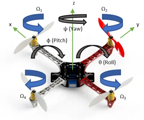
Figure 2.1 represents the quadrotor model used in this study and in previous work [27]. Here,

the motor configurations are shown, with the red propeller indicating the forward direction of the

(16)

Figure 2.1: Quadrotor Model

The rotational kinematics and translational dynamics are:

¨

φ =b1U2+a1θ˙ψ˙−a2θ˙Ωr

¨

θ =b2U3+a3φ˙ψ˙+a4ψ˙Ωr

¨

ψ =b3U4+a5φ˙θ˙

¨ x= U1

m(sinφ sinψ+ cosφ cosψ sinθ)

¨ y = U1

m(cosφ sinψ sinθ−cosψ sinφ)

¨ z = U1

m(cosφ cosθ)−g (2.1)

whereU1,U2,U3, andU4 are the thrust forces relating to heave, pitch, roll, and yaw, respectively.

The state variables φ, θ, ψ, x, y, z represent pitch, roll, yaw, x-position, y-position, and altitude,

respectively. where l is the arm length of the quadrotor and Jr is the rotor inertia. The system

parameters are obtained through physical modeling of a prototype experimental platform and

lit-erature search [28, 29]. The parameters assigned to the simulated system are shown in Table 2.1.

(17)

Table 2.1: System Parameters

m 0.98 kg g 9.81 m/s

l 0.17 m Ixx 0.01548 kgm2

Iyy 0.01565 kgm2

Izz 0.03024 kgm2

Jr 6e-5 kgm2

Kf 3.13e-5 N-s2

Km 3.13e-5 N-m-s2

U3 U4]T, the dynamics represented in (2.1) are written as:

˙

X =f(X) + Φ(X)_U(t) (2.2)

wheref(X) ∈ <12×1 _and _Φ(X) _{∈ <}12×4 _{is the input coefficient matrix. The system inputs are}

related to rotor speeds as:

         U1 U2 U3 U4          =         

Kf Kf Kf Kf

0 −Kf 0 Kf

Kf 0 −Kf 0

Km −Km Km −Km

                 

Ω2₁

Ω2₂

Ω2₃

Ω2 4          (2.3)

whereKf andKmare the aerodynamic force and moment constants respectively. The relative rotor

speedΩris the sum of rotor speeds:

Ωr =−Ω1+ Ω2 −Ω3+ Ω4 (2.4)

The parametersai andbi are the normalized and simplified inertia terms of the quadrotor,

(18)

a1 =

Iyy −Izz

Ixx

a2 =

Jr

Ixx

a3 =

Izz −Ixx

Iyy

a4 =

Jr

Iyy

a5 =

Ixx−Iyy

Izz

b1 =

l Ixx

b2 =

l Iyy

b3 =

1 Izz

(2.5)

2.2 Sliding Mode Control

The SMC attitude and altitude control laws from [27] are

U1 =

m

cosφcosθ[kzsgn(sz) +cz( ˙z−z˙d) +g+ ¨zd] U2 =

1 b1

[kφsgn(sφ) +cφ( ˙φd−φ) + ¨˙ φd+a2θΩ˙ r−a1θ˙ψ]˙

U3 =

1 b2

[kθsgn(sθ) +cθ( ˙θd−θ) + ¨˙ θd−a4φΩ˙ r−a3φ˙ψ]˙

U4 =

1 b3

[kψsgn(sψ) +cψ( ˙ψd−ψ) + ¨˙ ψd−a5φ˙θ]˙ (2.6)

The sliding surface is defined assi =ciei+ ˙ei, where tracking error isei =Xd,i−Xiwithi=φ,

θ, ψ and z. The equivalent and discontinuous control gains are ci and ki, respectively. These

control gains are selected through Particle Swarm Optimization (detailed in a later chapter) given

a finite range. The lower of the discontinuous gainski is determined from the maximum system

uncertainty to satisfy Lyapunov stability while the upper bound is selected to prevent excessive

control action [28, 30, 29, 31]. Ranges for the equivalent control gains ci were selected using a

(19)

Table 2.2: SMC Gain Search Bounds onki

Gain z φ θ ψ

min 0.0542 0.0542 0.0542 0.0542

max 200 30 30 30

Table 2.3: SMC Gain Search Bounds onci

Gain z φ θ ψ

min 0.05 0.05 0.05 0.05

max 10 10 10 10

The quadcopter inputs (2.6) control the roll, pitch, yaw, and altitude only while the x and

y horizontal positions are dependent on the attitude and heave U1. A multi-agent coordination

algorithm detailed in a later chapter is used to determine the virtual inputsux, uy, anduz which

are used to determine the desired rollθdand pitchφdsuch that

θd= tan−1

uxcosψ+uysinψ

uz+g

φd= tan−1

cosθd

uxsinψ−uycosψ

uz +g

(2.7)

and the modified altitude inputU1using

U1 =

m

(20)

CHAPTER 3 QUADCOPTER CONTROLLER GAIN OPTIMIZATION

Finding a suitable set of control gains for a system can be an ambiguous and time-consuming

process, particularly when optimal control methods, such as Linear Quadratic Regulators, are not

in use. This is especially true of highly nonlinear systems, such as quadcopters. In the previous

chapter Sliding Mode Control (SMC) was chosen for use on the quadcopter test platform due to it’s

robustness against system uncertainties and unmodeled dynamics. Stable and reasonable ranges

for the SMC gains were found through Lyapunov analysis and literature review. In this chapter

the method of Particle Swarm Optimization (PSO) is introduced and used to automatically tune

attitude and altitude SMC gains for a quadrotor experimental test platform. These results were

presented in [27].

3.1 Particle Swarm Optimization

A finite search space is established where each dimension is a parameter to be optimized. There

is no limit on the number of optimization variables. As such PSO is able to optimize a system

in an N-dimensional hyperspace. Artificial particles move through this search space to find an

optimal location. A particle’s N-dimensional location in the search space is used in a cost function

to determine that location’s fitness, a scalar value. In general optimization practice, a low cost is

considered favorable. Cost functions can take many forms; the Ackley, Easom, and McCormick

functions are commonly used for examining an optimization technique’s efficacy [32]. PSO iterates

to minimize the cost function until an ending condition is met. The most common end condition,

which is used in this study, is a set number of iterations.

Initialization- PSO begins by generating two initial test locations at random within the search

(21)

point to the other for each particle in the swarm. The cost at each of these locations is calculated

to provide seed data for each particle’s personal (or local) best tested location. From the swarm’s

set of personal best locations, a global best location is selected. The particles’ velocity, personal

best location, and the swarm’s global best location are used to determine where each particle will

move next in the search space.

PSO Equation- The general PSO equation for thej-th particle in a swarm at any stepkis

∆xj(k+ 1) =W(k)∆xj(k) +P(k)r1(j, k)[Pb,j(k)−xi(k)]

+G(k)r2(j, k)[Gb(k)−xj(k)]

xj(k+ 1) =xj(k) + ∆xj(k+ 1) (3.1)

where∆xj(k)and∆xj(k+1)are the current and next velocities,xj(k)andxj(k+1)are the current

and next positions, Pb,j(k) and Gb(k) are the personal and global best locations, respectively,

r1(j, k)andr2(j, k)are random values on the interval [0,1]generated for each particle at each step,

andW(k),P(k), andG(k)and the inertial, personal, and global weights which can be constant or

vary during the optimization process. Depending on these weights, different swarm behaviors can

emerge. Without loss of generality, the inertial, personal, and global weighting functions for this

study are chosen as

G(k) =e4( k kf−1)

P(k) = 1−G(k)

W(k) =e−4 k

kf _(3.2)

wherekf is the total number of steps. These functions are visualized in Figure 3.1. By having high

inertial and personal weight early in the optimization process, particles are encouraged to explore

the search space, seeking out new potential solutions. As the time step k increases, the personal

(22)

Figure 3.1: Visualization of varying PSO gains

of the way to the final step (solid black line in Figure 3.1). During this stage the particles tend

towards the global best solution, potential discovering new solutions due to the dominant inertial

weight. At roughly 83% completion (dashed black line in Figure 3.1), the global weight become

dominant, influencing the particles to converge to and refine a single optimal solution.

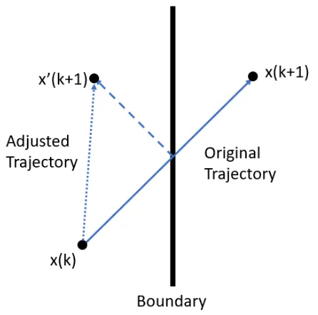
Boundary Handling - Several methods of ensuring particles remain in the search space were

considered including reflection, nearest, personal best, and random techniques. In [33], it was

found that the reflection boundary handling method resulted in the least sampling bias and will

be used for this study. Under this technique, when a particle’s next test position is outside of the

search space, the exterior trajectory is mirrored by the boundary resulting in a new next position

inside the search space. This is visualized in figure 3.2.

3.2 SMC Gain Tuning

The SMC control gains ki and ci where i = z, φ, θ, and ψ in the quadcopter control laws in

equation (2.6), reproduced below, are tuned using PSO. A set of gains take the place ofx in the

PSO equation (3.1) as the pseudo-location in the search space such thatxj(k) = [kzkφkθkψ czcφ

(23)

Figure 3.2: Visualization of reflect boundary technique

U1 =

m

cosφcosθ[kzsgn(sz) +cz( ˙z−z˙d) +g+ ¨zd] U2 =

1 b1

[kφsgn(sφ) +cφ( ˙φd−φ) + ¨˙ φd+a2θΩ˙ r−a1θ˙ψ]˙

U3 =

1 b2

[kθsgn(sθ) +cθ( ˙θd−θ) + ¨˙ θd−a4φΩ˙ r−a3φ˙ψ]˙

U4 =

1 b3

[kψsgn(sψ) +cψ( ˙ψd−ψ) + ¨˙ ψd−a5φ˙θ]˙ (2.6)

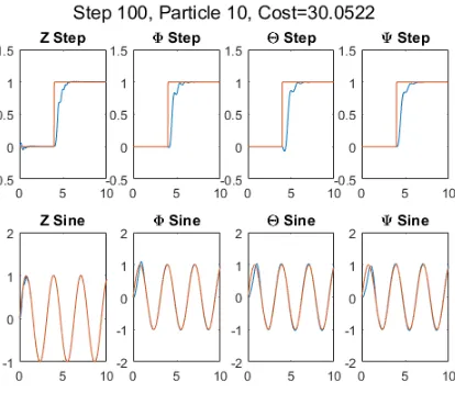
To determine the effectiveness or cost associated with of each set of gains, performance metrics

are calculated from step and sine wave tracking responses (without loss of generality) in each

respective degree of freedom. Performance metrics include time constants, steady state error,

tracking error, and controller effort. These are used to determine the costJj(k)such that

Jj(k) =

4

X

i=1

(ατ,iτi,j(k) +αE,iEi,j(k) +αT ,iTi,j(k) +αW,iWi,j(k) +αV,iVi,j(k)) (3.3)

(24)

y(τi,j(k)) = 0.632yss

Ei,j(k) =|yss−yd|

Ti,j(k) =

Z tf

0

|y(t)−yd(t)|dt

Wi,j(k) =

Z tf

0

|Ui,step|dt

Vi,j(k) =

Z tf

0

|Ui,sine|dt (3.4)

Hereiis each degree of freedom:z,φ,θ, andψ. τi,j(k),Ei,j(k), andWi,j(k)are the time constant,

steady state error, and control effort, respectively, from the step input response. ydand yd(t)are

a unit step and sine wave desired inputs, respectively. yssis the steady state value of the unit step

response. Steady state is reached if the absolute value of the first derivative of the response to a

step input reduces to a threshold chosen a priori before the final time of the simulation. Assuming

a first order response,τi,j(k)is then found as the time at which the step response reaches one time

constant, as defined in [34]. If the first derivative does not become smaller than the threshold before

the end of the simulation, it is assumed steady state is not reached and an arbitrarily largeτi,j(k)is

assigned. Ti,j(k)andVi,j(k)are the tracking error and control effort, respectively, from tracking a

sine wave. Each of these values are calculated such that they are always positive. Therefore, PSO

will work to minimize (3.3). Theαterms are combined normalizing and weighting gains.

Optimizations with this cost function are performed with simulations in both coupled and

de-coupled cases. In the de-coupled case, the simulated quadcopter receives command signals in all

degrees of freedom simultaneously. For example, step response maneuvers for altitude, roll, pitch,

and yaw are executed at the same time. In the decoupled case each degree of freedom is tested

independently while all others are told to remain at zero. Furthermore, optimizations with various

particle swarm sizes and iterations are performed and the results compared.

Other cost functions used in literature review are often more simple than equation (3.3). As

such the optimization results using the above cost function will be compared to optimizations using

(25)

Jj(k) =

4

X

i=1

αi,jMSEi,j(k) (3.5)

where MSEi,j(k)is the mean square error of a coupled step response of each degree of freedom

i=z,φ,θ, andψ. The resulting gains from optimizations using each cost function and simulation

technique are compared for consistency of results and time require to complete the optimization

process. The method which can produce consistent results in a comparatively reasonable amount

of time is used to obtain controller gains for implementation on a physical platform.

3.3 Simulation Results and Discussion

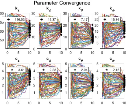
The Particle Swarm optimization of the SMC gain was performed with various combinations of

total iterationskf, numbers of particlesN, and the aforementioned cost functions. Sample result

are shown in Tables 3.1, 3.2, and 3.3 below. Additionally, cost figures, controller gain evolution

plots, and final step and sine tracking responses can be found in Appendix A.

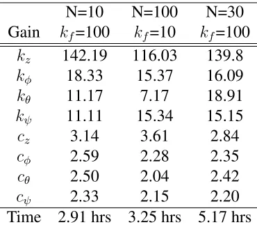
Table 3.1: PSO Tuned Quadcopter SMC Gains with Coupled Responses

N=10 N=100 N=30 Gain kf=100 kf=10 kf=100

kz 142.19 116.03 139.8

kφ 18.33 15.37 16.09

kθ 11.17 7.17 18.91

kψ 11.11 15.34 15.15

cz 3.14 3.61 2.84

cφ 2.59 2.28 2.35

cθ 2.50 2.04 2.42

cψ 2.33 2.15 2.20

Time 2.91 hrs 3.25 hrs 5.17 hrs

Through successive runs, several general observations are made. Firstly, it was seen that

with-out a sufficient number of steps in the optimization process, particles do not converge to a solution.

Conversely, allowing the optimization process to continue for a very large number of steps, such

as 1,000, does not produce any noticeable improvements to a final solution. Next, the number of

particles is found to greatly impact the swarm’s ability to find an optimal solution. With fewer

(26)

Table 3.2: PSO Tuned Quadcopter SMC Gains with Decoupled Responses

N=10 N=100 N=30 Gain kf=100 kf=10 kf=100

kz 195.02 1.44 172.6

kφ 25.04 17.74 15.66

kθ 10.03 28.67 15.12

kψ 20.71 15.83 17.31

cz 3.81 2.92 2.94

cφ 1.19 3.73 2.12

cθ 3.63 1.12 2.41

cψ 0.93 1.58 0.48

Time 11.77 hrs 12.18 hrs 35.1 hrs

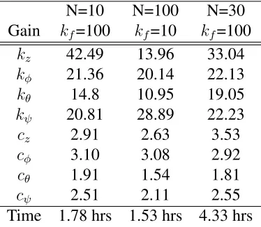
Table 3.3: PSO Tuned Quadcopter SMC Gains from Coupled Responses and MSE Cost

N=10 N=100 N=30 Gain kf=100 kf=10 kf=100

kz 42.49 13.96 33.04

kφ 21.36 20.14 22.13

kθ 14.8 10.95 19.05

kψ 20.81 28.89 22.23

cz 2.91 2.63 3.53

cφ 3.10 3.08 2.92

cθ 1.91 1.54 1.81

cψ 2.51 2.11 2.55

Time 1.78 hrs 1.53 hrs 4.33 hrs

for the optimization precess depends almost exclusively on the number of simulations performed.

Thus, more steps and more particles result in longer runtime. This also applies to the coupled

ver-sus decoupled simulation responses. Because the decoupled method uses independent simulations

for each degree of freedom, it takes a significantly longer amount of time to complete the

opti-mization using this method than using coupled responses. Furthermore no significant difference in

responses is seen between the two methods.

When considering the two cost functions presented in the previous section, it is found the

(27)

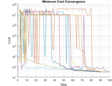
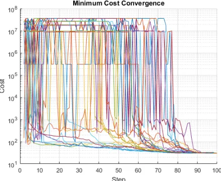
Figure 3.3: Cost convergence of 30 particle over 100 steps

resulting from Equation (3.3). This is most notable in step responses where significant oscillations

are present.

With these observations in mind, a balance of efficacy and efficiency is found for final tuning

of the Quadcopter SMC gains. Coupled responses are used with a swarm consisting of 30 particles

iterated for 100 steps using Equation (3.3) as the cost function. This setup yields consistent results.

Furthermore, particles exhibit the desired behavior from the selected inertial, global, and personal

weights as can be seen through the cost at each step for each particle in Figure 3.3. It is also

observed that the cost has discrete values when very large. This may be an artifact of the plotting

technique, a result of Sliding Mode Controller saturation, caused by cost parameter assignment

when bounds are exceeded, or a combination of these or other factors. The final gains used for

implementation on physical test platforms and in later simulations are given in table 3.4.

Table 3.4: Optimized SMC Gains

Gain z φ θ ψ

(28)

CHAPTER 4 ARTIFICIAL POTENTIAL FIELD SWARM COORDINATION

In this chapter a multi-agent control scheme capable of aggregating multiple autonomous

robotic agents into a formation as well as coordinating supplemental agents in a larger swarm

is presented. The algorithm is based on the leader-follower Artificial Potential Field-Sliding Mode

Control (APF-SMC) presented in [24]. Several modifications are introduced to the APF equation

to achieve formation aggregation and additional analysis is performed to prove certain assumptions

made in the original Lyapunov stability proof. These modifications were presented in [35]. The

new swarm coordinator is then proven stable following the form of the original work.

4.1 Leader-Follower Framework

The APF presented in [24] was built on attractive and repulsive forces as function of the distances

between each pairs of agenta. The attractive forces encourage swarm cohesion and aggregation

while the repulsive forces prevent agents from colliding and the swarm from collapsing into a

singularity. The potential field took the general form

∇xiVi(X) =

N

X

j=1

f_i,ja(kxi−xjk)(xi−xj)−fi,jr (kxi−xjk)(xi−xj)

+f_i,La (kxi−xLk)(xi−xL)−fi,Lr (kxi−xLk)(xi −xL) (4.1)

where Vi(X) is the potential at agent i as a function of the states of all agents X in the swarm

withN agents,xis the position of agentsiandj,fa_and_fr _{are the attractive and repulsive force}

(29)

Vi(X) = N X j=1 ka

2 kxi−xjk+ krr

2 e

−kxi−xjk

2

r

+ka,L

2 kxi−xLk+ kr,LrL

2 e

−kxi−xLk

rL _(4.2)

whereka andkr are attractive and repulsive forces respectively, r influences the area of effect of

the repulsive force,xi andxj are the positions of the agents iandj. This is the starting point for

the formulation of a decentralized swarm control algorithm with internal formation.

4.2 Formulation

4.2.1 Decentralization

By removing the leader components of equation (4.1) and separating the attractive forces from

the agent dynamics and assigning them to attractive nodes νk, which have their own prescribed

dynamics. The resulting general equation for a swarm ofN agents andM attractive nodes is

∇xiVi(X,N) =

M

X

k=1

f_i,ka (kxi−νkk)(xi−νk)− N

X

j=1

f_i,jr (kxi−xjk)(xi−xj) (4.3)

More specifically,

Vi(X,N) = M

X

k=1

kakxi−νkk+ N

X

j=1

kre−

k_xi−_xjk2

r (4.4)

where_Nis the states of all nodes in the potential field. Attractive nodes can be stationary in space

for regulation or move for tracking and can be used to aggregate the swarm into a specific formation

or structure. The repulsive forces remain dependent on agent dynamics to avoid collision.

4.2.2 Balancing Forces

During preliminary simulations using APF (4.4) to control a swarm of double-integrator point

masses, it was found that a zero-gradient region would form in the area enclosed by attractive

nodes due to symmetry in the attractive forces. An example of this can be seen in Figure 4.1a.

Furthermore, when more agents than nodes were in a swarm, often times no agent would reach

(30)

(a) Four agent, four node swarm trajectories,

dia-mond formation (b) Three agents, one node swarm trajectories

Figure 4.1: Multi-agent swarm aggregation

balancing forces of a lower magnitude than the attractive and repulsive forces already present,

these effects could be mitigated. That is, introducing a small linear repulsive force has the effect

of pushing agents towards nodes when in the aforementioned zero-gradient region. Introducing a

small Gaussian attractive force or "sink" holds agents at a node. With the inclusion of these forces

the APF becomes

Vi(X,N) = M

X

k=1

kakxi−νkk −kse

−k_xi−_νkk2

a

+

N

X

j=1

kre

−k_xi−_xjk2

r −k_lkx_i−x_jk

(4.5)

whereklis the long range repulsive gain,ksis the short range attractive gain, andainfluences the

area of effect of the short range attractive force..

4.2.3 Smoothness

To avoid singularities and potentially unstable dynamics, the APF must be smooth (i.e.

(31)

Figure 4.2: Artificial Potential Field visualization in a single dimension

in the gradient whenνk orxj is equal to xi. As such, these terms are modified with a hyperbolic

function with a "smoothness" factorcm. The final form of the proposed APF equation is

Vi(X,N) = M X k=1 ka p

kxi−νkk2+c2m−kse

−k_xi−_νkk2

a + N X j=1

kre

−k_xi−_xjk2

r −k_l q

kxi−xjk2+c2m

(4.6)

The profile of this APF in one dimension with one agent and one attractive node, both at the origin,

is shown in Figure 4.2. the attractive forcesfa _{and repulsive forces}_fr _{for the APF in the form of}

Equation (4.3), are

f_i,ka (kxi−νkk) =

ka

p

kxi−νkk2 +c2m

+2ks a e

−k_xi−_νkk2

a (4.7)

f_i,jr (kxi−xjk) =

2kr

r e

−k_xi−_xjk2

r + kl

p

kxi−xjk2+c2m

(4.8)

(32)

4.3 Equilibrium Distance

In Fabian et al. [24] it is assumed that there exists an equilibrium distance de where agents will

settle in relation to each other and the attractive and repulsive forces are equal. When considering

the overall swarm behavior it is useful to be able to assign an equilibrium distance such that agents

will settle with safe and proper space between themselves. As such, Equation (4.6) will be

ana-lyzed to find the analytical solution to the equilibrium distance as well as determine bounds and

expressions for gains to guarantee the specified equilibrium distance.

Definition 4.3.1(Equilibrium distance). There equilibrium distancedeis a distance away from an

agent where the attractive and repulsive forces balance each other satisfying fa

i,k(de) = fi,kr (de).

Moreover,fa

i,k(d)> fi,jr (d)for alld > deandfi,ka (d)< fi,jr (d)for all0< d < de

Definition 4.3.2(Lambert-W Function). Also called the product logarithm, the Lambert-W

func-tionW(z)is the inverse function off(z) =zez. That is,

Iff(z) = zez

ThenW(z) =f−1(z) (4.9)

Useful properties of the Lambert-W function used in the following analysis include

W(zez) = z (4.10) W(z)eW(z) =z (4.11)

Furthermore, for inputsx∈ <, the real output ofW(x)is divided into the principal branchW0

and the lower branchW−1 plotted in Figure 4.3 [36].

Assumption 4.3.1. A swarm governed by (4.6) will settle such that x¯ = ¯ν and that agents and

(33)

Figure 4.3: Real branches of the Lambert-W Function

Lemma 4.3.1. Consider a swarm of size N agents and M attractive nodes, with interactions

governed by (4.6) which satisfies Assumption 4.3.1. There exists an equilibrium distance

de =

−r 2 W−1

−r 2 K

2_e−2c

2

m r

−c2_m

1₂

(4.12)

and it is a local minimum in the potential field.

Proof. Applying Assumption 4.3.1 to Equation (4.6) and recognizing summation limits the APF

at agentibecomes

Vi(X,N) =M

ka

p

kxi−x¯k2+c2m−kse

−k_xi−x¯k2

a

+(N −1)

kre

−k_xi−x¯k2

r −k_lpkx_i−x¯k2+c2

m

(4.13)

Since an agent is at zero distance from itself, it cannot experience any repulsive forces from itself.

Therefore, the inter-agent forces sumN−1times for a swarm of sizeN.

Assigning the balancing force gains askl =δlka,ks =δskranda=r, like functions can now

be grouped together to yield

Vi(X,N) = [M −(N −1)δl]ka

p

kxi−x¯k2+cm2 + [(N −1)−M δs]kae

−k_xi−x¯k2

(34)

The equilibrium pointkxi−x¯k=deoccurs at the local minimum of the potential field such that

d dxi

Vi(X,N)

_k

xi−x¯k=de

= [M −(N−1)δl]ka

de

p

d2

e+c2m

+ [(N −1)−M δs]kr

−2de

r

e

−d2_e r = 0

(4.15)

The equilibrium distancedecan be solved for by first manipulating (4.15) into the formf(de)ef(de)

such that

[M −(N−1)δl]ka

de

p

d2

e+c2m

= [(N −1)−M δs]ka

2de

r

e

−d2_e r

[M −(N −1)δl]

[(N−1)−M δs)]

ka

kr

= 2 re

−d2_e r pd2

e+c2m

LetK be a value such that

K = [M −(N −1)δl] [(N −1)−M δs)]

ka

kr

(4.16)

Then,

K2 = 2 r

2 r d

2

e+c

2

m

e−2d 2 e r r 2K

2_e−2c

2

m r = 2

r d

2

e+c

2

m

e−2d 2

e r e

−2c2_m r

−r 2 K

2_e−2c

2

m

r = −2 (d

2

e+c2m)

r e

−2(d2_e+c2_m)

r (4.17)

Applying the Lambert-W function to both sides and recognizing the property Equation (4.10)

yields W ₋ r 2 K 2 e

−2c2_m r

= −2 (d

2

e+c2m)

r −r 2 W ₋ r 2 K 2 e

−2c2_m r

(35)

The equilibrium distance becomes

de =

₋ r 2 W ₋ r 2 K

2_e−2c

2

m r

−c2_m

1₂

(4.19)

Note that for de ∈ <+, W(−₂rK2e

−2c2_m

r ) must be negative and −r

2 W( −r

2 K

2_e−2c2m r )−c2

m must be

greater than zero. For Equation (4.19) to be a minimum, the APF described by Equation (4.6) must

have a positive second derivative (i.e., be concave up) atde.

Letµ= −₂rK2_e−2c

2

m

r andz2 = −r

2 W(µ), then Equation (4.19) may be written as

d2_e =z2−c2_m (4.20)

Taking the second derivative of Equation (4.14), evaluating it at kxi −x¯k = de, substituting in

Equation (4.20), and setting it greater than zero yields

[M −(N −1)δl]ka

"

z−z2−c2m

z

z2

#

+ [(N −1)−M δs]kre

−(z2−c2_m)

r

₋

2 r +

4 r2 z

2₋_c2

m

>0 (4.21)

Simplifying

K

1 z −

z2−c2_m z3

> 2 re

−z2 r e

c2_m r

1 +W(µ) + 2c

2 m r Kc 2 m

z3 >

2 r

eW(µ) 1 2 ec 2 m r

1 +W(µ) + 2c

2 m r Kc 2 m z2 1 −r

2 W(µ)

1₂ > 2 r µ W(µ) 1₂ ec 2 m r

1 +W(µ) + 2c

2 m r Kc 2 m

z2 >

2 r

r2 4K

2_e−2c

2 m r 1₂ ec 2 m r

1 +W(µ) + 2c

2 m r c2 m

z2 >

1 +W(µ) + 2c

2

m

r

−2c2

m

r < W(µ)

1 +W(µ) + 2c

2

m

r

(36)

−2c2_m r < W

2_{(µ) +}

1 + 2c

2

m

r

W(µ) (4.22)

Completing the square

−2c2

m

r +

1 4

1 + 2c

2 m r 2 <

W(µ) + 1 2

1 + 2c

2 m r 2 1 4

1− 2c 2 m r 2 <

W(µ) + 1 2

1 + 2c

2 m r 2 1 2

1− 2c 2 m r >

W(µ) + 1 2

1 + 2c

2 m r (4.23)

Considering all possible sign combinations resulting from the absolute value functions, to satisfy

the inequality

−r

2 W(µ)−c

2

m >0 (4.24)

necessary for a real positive equilibrium distancedefrom Equation (4.19), it is found thatW(µ)<

−1must be hold true. This is satisfied using the lower branch of the Lambert-W functionW−1(z)

forz ∈(−_e1,0). Therefore, the equilibrium distance

de =

₋

r 2 W−1

₋

r 2 K

2_e−2c2m r

−c2_m

1₂

(4.12)

is a local minimum of the potential field.

Lemma 4.3.2. Consider a swarm of size N agents and M attractive nodes, with interactions

governed by Equation (4.6) which satisfies Assumption 4.3.1. By selecting APF parameters such

thatde>0,ka>0,cm >0,δl < _NM₋₁,δs < N_M−1,cs >1, and calculated gains

kr =ka

[M −(N −1)δl]

[(N −1)−M δs)]

ecsc2m

γeγ

1₂

(37)

Where

γ = −c

2

m

d2

e+c2m

W−1

₋

1 ecs

(4.26)

r= 2c

2

m

W0(K2ecsc2m)

(4.27)

Here,

K = [M −(N −1)δl] [(N −1)−M δs)]

ka

kr

(4.16)

The resulting artificial potential field will have a local minimum at a distance de away from an

agent.

Proof. For realdein Equation (4.12)

−r 2 W−1

₋

r 2 K

2_e−2c

2

m r

−c2_m >0

W−1

₋

r 2 K

2

e

−2c2_m r

< −2c

2

m

r (4.28)

Note thatW−1(z)∈ <−for−1/e < z <0only. Therefore,

−1 e <

−r 2 K

2_e−2c

2

m r <0

0< r 2K

2_e−2c2m r < 1

e (4.29)

The design parametercs >1is introduced such that

r 2K

2_e−2c

2

m r = 1

ecs

(38)

satisfies the inequality (4.29). Equation (4.30) may be used to solve for the APF gainras follows:

r 2e

−2c2_m

r = 1

K2_ec

s

2 re

2c2_m

r =K2ec

s

2c2

m

r e 2c2_m

r =K2ec_sc2

m

2c2_m

r =W0 K

2_ec

sc2m

r= 2c

2

m

W0(K2ecsc2m)

(4.27)

To solve for one of the gains, Equations (4.30) and (4.27) are substituted into Equation (4.12)

yielding

de =

₋

c2

m

W0(K2ecsc2m)

W−1

₋

1 ecs

−c2_m

1₂

d2_e+c2_m

−c2

m

=

W−1

−1

ecs

W0(K2ecsc2m)

W0 K2ecsc2m

= −c

2

m

d2

e+c2m

W−1

−1 ecs

(4.31)

Defineγ such that

γ = −c

2

m

d2

e+c2m

W−1

−1 ecs (4.26) Then

W0 K2ecsc2m

=γ (4.32)

Applying the properties of the Lambert-W function yields

K2ecsc2m =γe γ

K2 = γe

γ

(39)

Substituting Equation (4.16) yields

[M −(N −1)δl]

[(N −1)−M δs)]

ka

kr

=

γeγ ecsc2m

1₂

Thus, the repulsive gainkrcan be defined such that

kr =ka

[M −(N −1)δl]

[(N −1)−M δs)]

ecsc2m

γeγ

1₂

(4.25)

Noting thatka∈ <+,

M −(N −1)δl >0

δl <

M

N−1 (4.33)

and

(N −1)−M δs >0

δs <

N−1

M (4.34)

The inequalities (4.33) and (4.34) must hold to yield a finite, real, kr. Thus, selecting APF

pa-rameters such that de > 0, ka > 0, cm > 0, δl < _NM₋₁, δs < N_M−1, cs > 1, and gains kr and r

from Equations (4.25) and (4.27), respectively, results in an Artificial Potential Field with a local

minimum at a distancede away from an agent.

4.4 Stability Under First-Order Dynamics

4.4.1 Swarm Centroid Dynamics

This stability analysis follows the process developed and presented by Fabian et al. in [24].

Consider the first order dynamics and control input

˙

(40)

and the APF

∇xiVi(X,N) =

M

X

k=1

X

j=1

with gains selected via Lemma 4.3.2. Node dynamics are assigned as

˙

νk=µk(t) (4.36)

which is chosen by the design engineer. The centroid of the attractive nodes is

¯ ν = 1

M

X

k=1

νk (4.37)

Assumption 4.4.1. Letfa_{(t) =}_fa

i,k(kxi−νkk). There existFa,F a

∈ <+_{such that}

Fa≤fa(t)≤Fa (4.38)

for allt. Furthermore, there existsFr ∈ <+_{such that}

0< f_i,jr (kxi−xjk)kxi−xjk< F r

(4.39)

Lemma 4.4.1. Consider a swarm of sizeN agents with dynamics described in Equation (4.35),

ofM attractive nodes with dynamics of Equation (4.36), with interactions governed by (4.6) and

with gains selected via Lemma 4.3.2. The swarm centroid dynamics are governed exclusively by

attractive node interaction forces such that the swarm centroidx¯dynamics follow

˙¯ x= −1

N

X

i=1

M

X

k=1

(41)

Proof. The swarm centroidx¯is defined as

¯ x= 1

N

X

i=1

xi (4.41)

Differentiating and applying the control law in Equation (4.35) yields

˙¯ x= 1

N

X

i=1

˙ xi =

1 N

N

X

i=1

ui (4.42)

˙¯ x= −1

N N X i=1 " _M X k=1

f_i,ka (kxi−νkk)(xi −νk)− N

X

j=1

f_i,jr (kxi−xjk)(xi−xj)

#

(4.43)

Note that inter-agent forces are equal and opposite for any given agent pair. That is, fr

i,j(kxi −

xjk) = −fj,ir (kxj −xik). Therefore, the second term of Equation (4.43) is zero, resulting in

Equation (4.40).

By applying Assumption 4.4.1 and recognizing the summation bounds to Equation (4.40), the

swarm centroid dynamics can be reduced to

˙¯

x=−M fa(t)(¯x−ν)¯ (4.44)

Lemma 4.4.2. Consider a swarm of sizeN agents with dynamics described in Equation (4.35), of

M attractive nodes with dynamics of Equation(4.36), with interactions governed by (4.6) and with

gains selected via Lemma 4.3.2. Ast → ∞the swarm centroidx¯will asymptotically approach a

hyperball around node centroidν¯of radius˜such that

˜

= µ(t)¯

M fa_(t). (4.45)

(42)

Proof. Consider the Lyapunov candidate

L(x) = 1 2˜e

T_˜_e _(4.46)

where ˜e = ¯x−ν¯ represent the vector from the agent swarm centroid x¯to the node centroid ν¯.

Taking the time derivative of the Lyapunov candidate yields

˙

L= ˙˜eTe˜= ( ˙¯x−ν)˙¯ T(¯x−ν) = ˙¯¯ xT˜e−ν˙¯T˜e (4.47)

By taking the time derivative of Equation (4.37) and applying Equation (4.36) we obtain the

aver-age movement of the nodes as

˙¯ ν = 1

M

X

k=1

µk(t) = ¯µ(t) (4.48)

By applying Lemma 4.4.1 and Assumption 4.4.1 yields

˙

L=−M fa(t)(¯x−ν)¯ T˜e−µ(t)¯ Te˜ ˙

L≤ −M fa(t)k˜ek2_{+ ¯}_µ(t)_k_e_˜_k _(4.49)

For stability and aggregationL˙ ≤0. Therefore

−M fa(t)ke˜k+ ¯µ(t)<0

k˜ek> µ(t)¯

M fa_(t) ≡˜ (4.50)

Thus, while the above inequality holds, the swarm centroid will converge to the node centroid.

Remark4.4.1. Rearranging Equation (4.50) as

¯

µ(t)< M fa(t)ke˜k (4.51)

and recall thatfa(t) = f_i,ka (kxi−νkk),e˜= ¯x−ν¯, and the APF gradient in the form of Equation

(43)

experienced by agents in the swarm. Therefore, from Equation (4.51), to maintain stability and

achieve swarm aggregation, the average node movement must be less than the total average

attrac-tive force. Moreover, if the nodes are stationary (i.e.,µk(t) = 0for allk = 1,2, ..., M), the swarm

centroidx¯will converge to the node centroidν¯.

4.4.2 Agent Dynamics

Theorem 4.4.3. Consider a swarm of sizeN agents with dynamics described in Equation (4.35),

ofM attractive nodes with dynamics of Equation(4.36), with interactions governed by (4.6) and

with gains selected via Lemma 4.3.2. The agents will converge to a hyperball around the swarm

centroid of radius

= (N −1)F

r

M fa (4.52)

Proof. Letei =xi−x¯, and consider the Lyapunov functionLi = 1₂eTi ei. Taking the time derivative

of the Lyapunov candidate along agent trajectories yields

˙

Li = ˙eTi ei = ( ˙xi−x)˙¯ Tei = (ui−x)˙¯ Tei (4.53)

LetL˙i be defined in terms ofΘ1,Θ2, andΘ3 such that

˙

Li = Θ1+ Θ2 + Θ3

Θ1 =

N

X

j=1

f_i,jr (kxi−xjk)(xi−xj)Tei

Θ2 =−

M

X

k=1

f_i,ka (kxi−νkk)(xi−νk)Tei

Θ3 =

1 N

N

X

i=1

M

X

k=1

f_i,ka (kxi−νkk)(xi−νk)Tei (4.54)

(44)

Θ1 = (N−1)F

r

keik

Θ2 =−M fa(t)(xi−νk)Tei

=−M fa(t)(ei+ ˜e)Tei

Θ3 =M fa(t)(¯x−ν)¯

=M fa(t)˜eTei

Thus,

˙

Li ≤(N −1)F r

keik −M fa(t)(ei+ ˜e)Tei+M fa(t)˜eTei

≤(N −1)Frkeik −M fa(t)eTi ei

≤(N −1)Frkeik −M fa(t)keik2

≤ keik

(N −1)Fr−M fa(t)keik

(4.55)

Sincekeik ≥0, the time derivative of the Lyapunov candidate is negative if

keik>

(N −1)Fr

M fa_(t) ≡ (4.56)

Thus, while keik > , agents will be attracted to the set point ei = xi −x¯ = 0and converge

asymptotically to the hypersphere of radiusaround the swarm centroidx¯.

Corollary 4.4.3.1. Given proper APF gain selection, while the distances from an agent to each

at-tractive nodekxi−νkkand the distances between agentskxi−xjkare greater than the equilibrium

distancede, agents will converge towards the swarm centroidx¯.

Proof. Consider Theorem 4.4.3 at Equation (4.54). By recognizing summation limits, applying

Assumption 4.4.1 and similarly assuming there exists a function fr(t) wherefr(t) = f_i,jr (kxi −

(45)

˙

Li ≤(N −1)fr(t)eTi ei−M fa(t)(ei+ ˜e)T +M fa(t)˜eTei

≤[(N −1)fr(t)−M fa(t)]keik2 (4.57)

Thus Lyapunov stability is achieved when

[(N −1)fr(t)−M fa(t)]<0

(N −1)fr(t)< M fa(t) (4.58)

Considering the state dependent force Equations f_i,ka (kxi −νkk)andfi,jr (kxi −xjk)in Equation

(4.58), and recalling that using gains determined via Lemma 4.3.2 satisfy Lemma 4.3.1i t is found

that whilekxi−νkkandkxi−xjkare greater thande, Equation (4.58) is satisfied and the controller

is stable in the sense of Lyapunov forei =xi −x¯→0ast→ ∞.

From Lemmas 4.4.1 and 4.4.2 and Theorem 4.4.3, it is proven that agents converge to a

hy-perball around the swarm centroid x¯, which converges to the centroid of the attractive nodes.

Therefore, the agents converge to a hyperball around the node centroid.

4.5 Stability Under General Dynamics

With the first order system and input described in Equation (4.35) shown to be stable, these results

can be extended to general higher order systems using Sliding Mode Control. This analysis is

based on [24] and, as such, requires the same assumptions and has the same process as follows.

Consider general agent dynamics governed by

Mi(xi)¨xi+gi(xi,x˙i) = ui (4.59)

whereMi(xi) is the inertial matrix for agent iand gi contains any higher order or nonlinear

(46)

Assumption 4.5.1. For all agentsi= 1,2, ..., N

Miky2k ≤yTMi(xi)y≤Miky2k<∞ (4.60)

for real scalars

0< Mi < Mi <∞ (4.61)

and any arbitraryy

Assumption 4.5.2. For allt≥0the time derivatives of the force functions must be such that

˙

f_i,ka (kxi−νkk)kxi−νkk ≤Γa(X,N)for alli, k

˙

f_i,jr (kxi−xjk)kxi−xjk ≤Γr(X)for alli, j (4.62)

whereΓa_and_Γr_{are state dependent upper bounds, however, global bounds are sufficient.}

Assumption 4.5.3. For all {i, j} and {i, k} pairs, where i = 1,2, ..., N, j = 1,2, ..., N, and

k = 1,2, ..., M, the potential field gradients are bounded by

k∇xiV(X,N)k ≤α(X,N)

k∇xj[∇xiV(X,N)]k ≤β(X,N)

k∇νk[∇xiV(X,N)]k ≤γ(X,N) (4.63)

whereα(_X,_N),β(_X,_N), andγ(_X,_N)are known, finite functions of the agent and node states.

Assumption 4.5.4. x˙i(0) = 0fori= 1,2, ..., N

Theorem 4.5.1. Consider a swarm of sizeN agents with dynamics described by Equation (4.59),

(47)

Potential Field described by Equation (4.6), gains selected via Lemma 4.3.2, and which satisfies

the aforementioned assumptions. Let the control input for agentibe

ui =−Ki(X,N)sign(si) +gi(x, xi) (4.64)

with gain

Ki(X,N)> Mi(xi)(Ji(X,N) +i) (4.65)

for some >0, where

Ji(X,N) =M γ(X,N)(α(X(0),N(0)) +α(X,N))

+N β(_X,_N)(α(_X(0),_N(0)) +α(_X,_N))

+MΓa(_X,_N)−(N −1)Γr(_X) (4.66)

and sliding manifold

si = ˙xi+∇xiV(X,N) (4.67)

Then sliding mode occurs in allsi and

˙

xi =−∇xiV(X,N) (4.68)

is satisfied in finite time.

Proof. For the Lyapunov candidate

Λi =

1 2s

T

i si (4.69)

sliding mode occurs in finite time if

˙

(48)

for somei > 0, also know as the reaching condition. Taking the time derivative of the sliding

manifold yields

˙

si = ¨xi+

d

dt∇xiV(X,N)

=Mi(xi)−1ui−Mi(xi)−1gi(xi,x˙i) +

d

dt∇xiV(X,N) (4.71)

Thus,

sT_i s˙i =sTi

Mi(xi)−1ui−Mi(xi)−1gi(xi,x˙i) +

d

dt∇xiV(X,N)

(4.72)

Recalling that

∇xiVi(X,N) =

M

X

k=1

X

j=1

and taking the time derivative and applying the product rule yields

d

dt∇xiVi(X,N) =

M

X

k=1

∇νk[∇xiV(X,N)] ˙νk+

N

X

j=1

∇xj[∇xiV(X,N)] ˙xj (4.74)

+

M

X

k=1

˙

X

j=1

˙

As stated in [24], it is shown in [37] that

k

M

X

k=1

∇νk[∇xiV(X,N)] ˙νkk ≤M γ(X,N)(α(X(0),N(0)) +α(X,N))

k

N

X

j=1

(49)

Therefore,

kd

dt∇xiV(X,N)k ≤M γ(X,N)(α(X(0),N(0)) +α(X,N)) +N β(_X,_N)(α(_X(0),_N(0)) +α(_X,_N))

+MΓa(_X,_N)−(N −1)Γr(_X) (4.77)

and

kd

dt∇xiV(X,N)k ≤Ji(X,N) (4.78)

Then

˙ Λi ≤sTi

Mi(xi)−1ui−Mi(xi)−1gi(xi,x˙i) +Ji(X,N)

≤sT_i Mi(xi)−1(−Ki(X,N)sign(si) +gi(x, xi))−Mi(xi)−1gi(xi,x˙i) +Ji(X,N)

≤sT_i −Mi(xi)−1Ki(X,N)sign(si) +Ji(X,N)

(4.79)

LetKi(X,N)be such that

Ki(X,N)> Mi(xi)(Ji(X,N) +i) (4.80)

Then

˙

Λi ≤ −sTi

(Ji(X,N) +i)sign(si)−Ji(X,N)

≤ −ksik(Ji(X,N) +i)−sTi Ji(X,N)

≤ −ksik(Ji(X,N) +i) +ksikJi(X,N) (4.81)

Which results in

˙

(50)

Thus, the reaching condition is met, sliding occurs in finite time and the control input described in

Equation 4.64 for general dynamics described in Equation (4.59) is stable in the sense of Lyapunov.

4.6 Simulation Results and Discussion

4.6.1 Quadcopter Swarm

Using the quadcopter model detailed in Equation (2.1) for a homogeneous swarm, attitude

Sliding Mode Control Equation (2.6), modified altitude input Equation (2.8), desired roll and pitch

Equations (2.7), and artificial potential field multi-agent position controller given as

ui =−Kisat(si) (4.83)

for agent i whereui = [u_i,x u_i,y u_i,z]T are the virtual position inputs, Ki = [K_x K_y K_z]T

are the APF-SMC discontinuous gains which is the same for each agent, the signum function is

replaced with a saturation function to reduce chattering and operate element wise on the sliding

manifoldsi = [si,x si,y si,z]T, and

si = ˙ˆxi+∇xˆiVi(X,N)

Vi(X,N) = M

X

k=1

ka

p

kxˆi−νkk2+c2m−kse

−k_xiˆ−_νkk2

a

+

N

X

j=1

kre

−k_xiˆ−_xjˆ k2

r −k_l q

kxˆi−xˆjk2+c2m

(4.6)

where xˆi = [xi yi zi]T is the position of agent i. Without loss of generality, gains used in

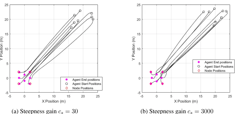
Equation (4.6) for simulations were chosen as ka = _M4 , de = 3, cs = 30, ck = 0.5, a = r,

δl = 0.2M_N, and δs = 0.2_MN, with gains kr and r are determined through Lemma 4.3.2. The

(51)

Figure 4.4: Trajectories aggregating a 4-node formation

Figure 4.4 shows a group of 4 quadcopters (N = 4) with initial conditions:

x0 =

        

25 20 0

15 20 0

20 25 0

20 15 0

         (4.84)

and 4 stationary attractive nodes (M = 4) stationary atν:

ν =         

2 2 5

−2 2 5

−2 −2 5

2 −2 5

         (4.85)

It is observed that all agents flock towards the attractive nodes without collision and settle in the

intended formation without assigning specific agents of specific nodes.

(52)

Figure 4.5: Trajectories tracking a 2-node formation

ˆ x0 =

        

5 0 0

−5 0 0

0 5 0

0 −5 0

         (4.86)

and 2 attractive nodes (M = 2) with trajectories

ˆ ν(t) =



 

sin(0.5t) + 3 0.25t 5

sin(0.5t)−3 0.25t 5





 (4.87)

It can be seen that 2 quadcopters successfully track the moving nodes on their trajectories while

the additional agents follow the swarm centroid while maintaining separation.

Figures 4.6a through 4.7 show a swarm of 4 quadcopters (N = 4) with initial conditions:

x0 =

        

5 0 0

−5 0 0

0 5 0

0 −5 0

(53)

(a) Trajectories aggregating a 2 node formation be-fore single-agent failure

(b) Trajectories aggregating a 2 node formation with single-agent failure

Figure 4.6: Quadcopter swarm trajectories before and after agent failure

and 2 attractive nodes (M = 2) stationary at:

ν(t) =



 

3 0 5

−3 0 5





 (4.89)

The agent trajectories during initial swarm aggregation can be see in Figure 4.6a. At t = 30

seconds in the simulation, Agent 1 is artificially sent out of the formation in the negativezdirection.

The full trajectories can be seen in Figure 4.6b. For clarity, Figure 4.7 shows the x, y, and z

coordinates versus time on separate plots for all agents. When Agent 1 exits the formation, it

is observed that the remaining agents adjust themselves to re-aggregate the desired formation.

That is, Agents 3 moves to the now vacant node while Agent 4 finds a new equilibrium in the

swarm. Agent 2 remains stationary during the re-aggregation. This is achieved solely through the

interactions from the artificial potential field, noting that no assignments for agents to nodes are

madea priori.

The Artificial Potential Field method of multi-agent coordination may also be used for

(54)

Figure 4.7: Agent coordinates aggregating a 2 node formation with single-agent failure

(a) Agent trajectory in space

(b) Agent positions in x, y, andz directions versus time

(55)

within a threshold distance of the current waypoint, the attractive node changes to the next desired

location. A waypoint list

w=                             

0 0 5

0 10 5

5 10 5

5 −10 5

10 −10 5

10 10 5

15 10 5

15 −10 5

20 −10 5

20 10 5

                             (4.90)

contains the corners of a basic lawnmower path. The waypoint iterates when the agent is within 1

meter of the current target. For this simulation gains were selected aska = 10,de = 2,cs = 100,

ck = 10, a = r, δs = 0.2, and δl = 0.2. Gains kr and r are determined through Lemma 4.3.2.

The discontinuous gains are selected asKi = [2 2 20]T. Figure 4.8 shows simulated quadcopter

initially at (0, 2, 0) moving towards each successive waypoint, following the lawnmower path.

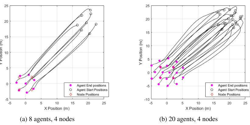
4.6.2 Point-Mass Swarms

Swarm Aggregation

Due to large computational loads, simulating numerous quadcopters requires a significant

amount of time. As such, having shown proof of concept with relatively small quadcopter swarms,

to lessen the computational load, larger swarms are simulated with simple point-mass, double

inte-grator dynamicsx¨ˆi =ui. Furthermore, while it is shown in the previous section that the APF-SMC

multi-agent coordinator is capable of controlling agents in three dimensions, the following

simu-lations will be restricted to horizontal movement and interaction through the APF to thex-yplane

to improve interpretability of Figures. APF gains ka = _M4 , de = 3, cs = 30, ck = 0.5, a = r,

Quadcopter Attitude Control Optimization and Multi-Agent Coordination

University of New Hampshire

University of New Hampshire Scholars' Repository

Quadcopter Attitude Control Optimization and

Multi-Agent Coordination

John McCormack

TABLE OF CONTENTS

LIST OF TABLES

LIST OF FIGURES

ABSTRACT

Quadcopter Attitude Control Optimization and Multi-Agent Coordination

by

John McCormack

CHAPTER 1

INTRODUCTION

1.1

Particle Swarm Optimization

1.2

Robotic Swarm Control Methods

1.3

Organization

CHAPTER 2

QUADCOPTER MODELING AND CONTROL

2.1

Quadcopter Model

2.2

Sliding Mode Control

CHAPTER 3

QUADCOPTER CONTROLLER GAIN OPTIMIZATION

3.1

Particle Swarm Optimization

3.2

SMC Gain Tuning

3.3

Simulation Results and Discussion

CHAPTER 4

ARTIFICIAL POTENTIAL FIELD SWARM COORDINATION

4.1

Leader-Follower Framework

4.2

Formulation

4.3

Equilibrium Distance

4.4

Stability Under First-Order Dynamics

4.5

Stability Under General Dynamics

4.6

Simulation Results and Discussion