Printed in The Islamic Republic of Iran, 2011 © Shiraz University
MULTI–OBJECTIVE TRANSMISSION EXPANSION PLANNING
USING FUZZY–GENETIC ALGORITHM
*M. SHIVAIE
**1M. S. SEPASIAN
1AND M. K. SHEIKH–EL–ESLAMI
21Dept. of Electrical and Computer Engineering, Power & Water University of Technology (PWUT),
Tehran, I. R. of Iran, Email: [email protected]
2Dept. of Electrical and Computer Engineering, Tarbiat Modares University (TMU), Tehran, I. R. of Iran
Abstract– In this paper a new framework is presented for multi–objective Transmission Expansion Planning (TEP). This framework is based on a multiple criteria decision making whose fundamental elements are REliability and MARKet (REMARK). Investment cost, congestion cost, Users' Benefit (UB) and Expected Customer Interruption Cost (ECOST) are considered in the optimization as four objectives. The proposed model is a complicated non–linear mixed–integer optimization problem. A hybrid Genetic Algorithm (GA) and Quadratic Programming (QP) is used, followed by a Fuzzy Sets Theory (FST) to obtain the final optimal solution. The planning methodology has been demonstrated on the 6–machine 8–bus test system to show the feasibility and capabilities of the proposed algorithm. Also, in order to compare the historical expansion plan and the expansion plan developed by the proposed methodology, it was applied to the real life system of the northeastern part of Iranian national 400–kV transmission grid.
Keywords– Electricity market, fuzzy sets theory (FST), genetic algorithm (GA), quadratic programming (QP), transmission expansion planning (TEP)
1. INTRODUCTION
Transmission Expansion Planning (TEP) is an important component of power system planning. It determines the characteristics and performance of the future electric power network and influences power system operation directly [1]. Generally, TEP can be classified as static transmission planning or dynamic transmission planning [2]. In recent years, and, at the same time restructuring in the power industry, various studies have been carried out into the TEP in electricity markets and its adjustment to market conditions [3]. Due to the emergence of new challenges in the electricity market such as more uncertainties and a more competitive environment, new methods have been presented to minimize the risk of planning and also satisfy the market–based criteria. Probabilistic tools such as Monte Carlo simulation [4] are very prevalent methods for modeling uncertainties in planning processes. In [5–7], random uncertainties are considered by probabilistic density function, whereas non–random uncertainties are modeled using scenario technique. In order to increase the competition among the participants of the electricity market, new criteria are introduced to provide a fair environment for network users. In [5], congestion cost is used to measure the competitiveness degree of an electricity market. From another viewpoint, maximizing the social welfare can be used as a proper criterion to encourage the competition between the participants. The optimization of the aggregate social welfare according to the different levels of demand scenarios in a pool–based electricity market are formulated as a mixed integer linear programming in [8]. Reliability assessment is one of the most important parts of TEP [9–10]. Expected energy not supplied, computed for each period of planning has been applied in [11] as a reliability criterion. Since the expected energy not supplied computational process is time consuming, the proposed
algorithm is not applicable in large systems. The N–1 criterion is used in [12] for the contingency analysis to calculate the loss of load cost. In [13–14] the security assessment of the network has been delayed after the end of the planning process (second phase). The best ones from the rest of the candidate lines are added into the network until no overloading happens in the system. It may severely jeopardize the purpose of ‘‘optimal planning”. Also, in [15–16], a probabilistic criterion, known as expected customer interruption cost due to transmission constraint is presented to evaluate the value of reliability. From the above investigation into TEP methods, some drawbacks in modeling such as insufficiency of objective functions and ignorance of value–based reliability assessment can be seen. This paper focuses on defining a multi–objective framework to handle different stakeholders’ objectives with a cost–benefit approach. This framework is based on a multiple criteria decision making whose main elements are REliability and MARKet (REMARK). In this model, the standpoint is taken that TEP should serve its users, so the benefit of both participants in the market and investment cost are considered as economic criteria for the electricity market [13, 17] and the congestion cost of the network as a factor for encouraging market competition [18]. Also, a probabilistic criterion, Expected Customer Interruption (ECOST) was considered to evaluate the value of reliability [15–16]. Therefore, effective factors of TEP are integrated in competitive environments and are formulized as a multi–objective model. The proposed model is a complicated non–linear mixed–integer optimization problem. A hybrid Genetic Algorithm (GA) and Quadratic Programming (QP) are used followed by a Fuzzy Set Theory (FST) to obtain the final optimal solution. The discrete decision–making variables of the expansion are optimized by GA, while QP optimizes the continuous plans. The planning methodology has been demonstrated on the 6–machine 8– bus test system [19–20] and the real life system of the northeastern part of Iranian national 400–kV transmission grid [21] to show the feasibility and capabilities of the proposed algorithm. The advantages of this paper compared to the previous works in the field of TEP algorithm are:
Considering a new value based reliability TEP process using a multi–objective approach.
Considering the power markets’ requirements and encouraging and facilitating competition among market participants.
Total Congestion cost index is used as a proper criterion for measuring the competitive degree of each plan.
The planner preferences of different planning criteria have been considered in choosing the final plan. The remainder of this paper is organized as follows. Section 2 describes formulation of power–pool operation. The proposed TEP model is presented in section 3. The solution algorithm of the proposed model and case studies are presented in section 4 and 5, respectively. The resulted conclusions are then presented in section 6.
2. FORMULATION OF POWER–POOL OPERATION
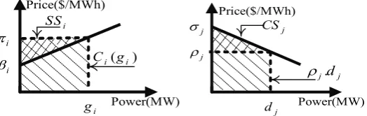
The mathematical formulation of the pool operation in the electricity market is presented in this section. This becomes the operational problem of our TEP problem. The independent system operator performs this market–clearing process considering the bids submitted by generators, consumers, and transmission constraints [13, 17]. In a pool model, each market participant submits an hourly price bid in the form of marginal cost or marginal benefit functions [$/MWh]. The supply bids are assumed to be linear with an upward slope and consumer bids are assumed to be linear with a downward slope. Therefore, for a particular generator i, the price and quantity supplied is defined as Eq. (1).
i i igi
π =β +α ,gi ≤gi ≤gi (1)
operating point (gi , dj), where:
2
1 2 ( )
i i i ig i i i
C g = α +β g +ψ (2)
The generation cost difference with the hachured part in Fig. 1 is just in the constant value Ψi. Similarly, for a particular consumer j, price bid is defined as Eq. (3).
j j jdj
ρ =σ +δ ,dj ≤dj ≤dj (3)
The demand bid of Fig. 1 describes the Consumer’s Surplus (CSj) and benefit function of consumer j
(Bj(dj)), where:
2 1 ( )
2
j j j j j j j
B d = δ d +σ d +ξ (4)
The benefit function difference with the hachured part in Fig. 1 is just in the constant value ξj.
i π
i β
i
g
( ) i i
C g
i
SS Price($/MWh)
Power(MW)
j
σ
j
ρ
j d
. j dj ρ j CS
Power(MW) Price($/MWh)
Fig. 1. Supply and demand side bid representation
a) Objective function
In electricity markets with power–pool structure, LMP is one of the common methods for power pricing determination. In this model, power system operating is carried out by maximizing Social Welfare Function (SWF) [13, 17, 22]. This function is formed by the total benefit function minus the total apparent generation cost which is presented in Eq. (5).
Maximize :
( ) ( )
j j i i j J i I
SWF B d C g
∈ ∈
= ∑ − ∑
(5)
Subject,to :
j i 0
j J∑∈ d −i I∑∈ g = (6)
i i i
g ≤g ≤g ,∀ ∈i I (7)
j j j
d ≤d ≤d ,∀ ∈j J (8) ,,
l l l
f f f l L
− ≤ ≤ ∀ ∈ (9)
3. MATHEMATICAL MODEL OF MOTEP
The proposed model optimizes objective functions simultaneously, namely the investment cost, the congestion cost, the users' benefit and the ECOST. The MOTEP has been formulized below:
Minimize:
1 m
F =ICI
(10)
2 p. m
p P
F D TCCI
∈
= ∑ (11)
4 m
F =ECOST (12) Maximize:
3 p.m
p P
F D ΔSWF
∈
= ∑ (13)
Subject to constraints (6) - (8) and:
0 T
S F +G −D =
(14) 0
( )( ) 0
sr sr sr sr s r
f −γ η +η θ −θ = , ( , )∀ s r ∈ Ω
(15) 0
( )
sr sr sr sr
f ≤ η +η f , ( , )∀ s r ∈ Ω
(16)
, ,
, ,
0≤ηsr ≤η ηsr sr is integer variable , ( , )∀ s r ∈ Ω
(17) 0
( ),,
sr sr sr sr
Y = − y +η τ s ≠r , ( , )∀ s r ∈ Ω
(18) 0
0 ( ) ,,
ss s sr sr sr r s
Y y y η τ s r
∈
= + ∑ + ≠ , ( , )∀ s r ∈ Ω
(19)
Equation (14) and Eq. (15) are load flow relationships and Eq. (16) points to the power flow limitations. Eq. (17) requires transmission line expansion within the bounds of maximum line addition. Eq. (18) and Eq. (19) simply update the network admittance matrix with expansion [15–16].
a) Investment cost index (ICI)
The criterion studied in this paper is the investment cost index. By considering the plan m in the ICI, a criterion is defined as "ICI for the plan m" according to the Eq. (20) [21]. If we suppose that this model utilizes a scheduled long term loan to clear the enforced investment costs, the annual investment cost for candidate facilities can be calculated as follows:
( , )
(1 ) [ . ]
(1 ) 1 T m s r sr sr T
ICI CL η ν ν
ν
∈Ω
+
= ∑ ×
+ − (20)
whereICImand ∑[CLsr.ηsr] are stated for the annual capital investment and the total capital investment of any new facility, respectively.
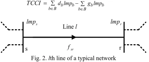
b) Total congestion cost index (TCCI)
in planning horizon and will try to minimize it as one of the problem objectives. The congestion cost of the lth line, shown in Fig. 2 is as follows [20]:
( ) ,
l r s sr
CCI = lmp −lmp f ∀ ∈l L (21)
where lmps is the LMP at bus s and lmprthe LMP at bus r in $/MWh. Total congestion cost index for all network lines at the planning horizon is formulated as:
( )
l r s sr l LCCI l L lmp lmp f
TCCI
∈ ∈
∑ = ∑ −
= (22)
So far considering the expansion plan m in congestion cost, according to Eq. (22), is defined as the "TCCI for the plan m" according to the Eq. (23).
m
m l
l L
TCCI CCI
∈
= ∑ (23)
It is proved that the total congestion cost of the network is equal to the sum of consumers’ payments minus the sum of generators income [9], i.e.:
b b b b b B b B
d lmp g lmp
TCCI
∈ ∈
∑ − ∑
= (24)
sr
f Line,l
s r
s
lmp lmpr
Fig. 2. lth line of a typical network
c) Users' benefit (UB) due to transmission expansion planning
The third criterion that has been studied in this paper is the users' benefit. The hourly benefit for generator i is defined as Eq. (25) [13, 17].
( )
( ) ( ). ( )
i h i h i h i g ti h
SB t =lmp t g t −C ⎡⎣ ⎤⎦ (25)
and total benefit in time T is equal to:
( ) i h i
th TSB t
TSB ∈
∑
= (26)
By network expansion and congestion decrease, the market conditions will improve and also LMPs will change for all users. This may lead to the UB change in the electricity market. Thus, the benefits of the expansion plan m for generator i will be calculated by Eq. (27).
, , , , , ,
0
, ( ) ( )
h h
m
i h i h
i m
t T t T
W ith Expansion Plan m Without Expansion Plan m
SB t SB t
SB
∈ ∈
∑ ∑
= −
14243 14243
(27)
Also, the hourly benefit for consumer j is defined as Eq. (28).
( )
( ) j ( ). ( )
j h j d th j h j h
CB t =B ⎡⎣ ⎤ −⎦ lmp t d t
(28)
and total benefit in time T is equal to:
( ) j h j
th TCB t
TCB ∈
∑
For similar reasons, the benefit of the expansion plan m for the consumer j will be calculated as: , , , , , , 0 , ( ) ( ) h h m
j h j h
j m
t T t T
With Expansion Plan m W ithout Expansion Plan m
CB t CB t
CB ∈ ∈ ∑ ∑ = − 14243 14243 (30)
The TEP problem is very difficult and complicated to solve because of the numerous inputs for every hour and for every user. Thus, the numerous calculations required and the problem of predicting the prices can be reduced by using the daily and seasonal patterns of the users. So, by dividing the time T to some distinct patterns, Eq. (27) can be rewritten in the following form.
, .
p p i m m i
p PD SB
SB
∈
∑ Δ
= (31)
Similarly, for the consumer j, we have:
, .
p p j m p PD mCBj
CB
∈
∑ Δ
= (32)
By using Eq. (25) and Eq. (28), the UB can be separated into the following elements.
( ) ( )
i h j h Tot i I
j J SB t CB t
UB
∈ ∈
∑ − ∑
= (33)
[ ( )] [ ( )]
( ). ( ) ( ). ( ) j j h i i h
j J i I
j h j h i h i h
j J i I
B d t C g t
lmp t d t lmp t g t
∈ ∈ ∈ ∈ = ∑ − ∑ − ∑ − ∑ ⎛ ⎞ ⎜ ⎟ ⎝ ⎠ ⎛ ⎞ ⎜ ⎟ ⎝ ⎠
The first term of Eq. (33) is the social welfare function due to expansion. In each year, this function is gained by solving operation Eq. (5) to Eq. (9) and after, updating Eq. (9). The second term in Eq. (33) is the same as the network users’ congestion cost which was described earlier as a decision making criterion. Thus, according to Eq. (33), in order to consider the expansion plan m in the UB, a criterion is defined as "the users' benefit for plan m" as follows.
. Tot p
mUB p P∈ D mSWF
Δ = ∑ Δ
(34)
d) Expected customer interruption cost (ECOST)
In a general classification and by using reliability criteria, there are two common TEP models. In the first model, the reliability criteria are considered as a constraint [23]. But in the second model, planning is based on the value of reliability and the sum of the costs and unreliability cost is optimized as objective function [16]. Thus, by considering reliability laws which change from a constraint to an object in competitive environments and by considering that one of the important objections of the network expansion is minimizing the electricity interruption damage, the expected customer interruption cost is the fourth criterion which is studied in this paper. So, the optimal values of load curtailment are calculated by using a new linear optimization problem as is shown in Eq. (35) to Eq. (39) [15–16].
Minimize :
( ) e
jn jn e jn
j J n N∑ ∑∈ ∈ χ ×c t ×w (35)
Subject,to:
max
' '
' ,
( e ) e . e , ,
b bn bn bb b
n N b B
g d Y θ b B e E
∈ ∈
− ∑ − χ = ∑ ∀ ∈ ∀ ∈
(36)
'( ') ,, ,
e e e
b l
bb b
Y θ θ f l L e E
− − ≤ ∀ ∈ ∀ ∈
'( ' ) ,, ,
e e e b l bb b
Y θ θ f l L e E
− − ≤ ∀ ∈ ∀ ∈ (38) max
0≤ χ ≤ejn djn ,,∀ ∈n N,∀ ∈ ∀ ∈j J, e E (39)
As was mentioned earlier, load curtailment is done by ISO and has different purposes. Weight coefficient
jn
w in Eq. (35) determines the load shedding purpose. In the proposed load curtailment philosophy, each load is divided into n parts based on the existing customer classes (sectors). Each sector has a Sector Customer Damage Function (SCDF) [15–16]. In each state with given outage duration, the unit interruption cost of sector n at bus j (cjn) is determined by use of the SCDF of each sector in terms of $/kW. cjnshould be updated in each scanned state based on the outage duration of that state. The sum of the product of the curtailed load of sector n at bus j ( e
jn
χ ) and cjnis the Load Curtailment Cost (LCC) of each state which is minimized as an objective function in the state evaluation process. The State Probability (SP) and the LCC of all scanned failure states are used to calculate ECOST as follows:
e e e E
ECOST LCC sp
∈
= ∑ × (40)
4. SOLUTION ALGORITHM
a) Genetic algorithm (GA)
Genetic algorithm starts with a set of initial solutions which are randomly selected from the feasible solution space. Assigning fitness to each solution and consequently ranking them, the population evolves through several operations such as reproduction, crossover and mutation to obtain the final optimal solution. Regarding useful properties of GA for solving multi–objective optimization problems such as the ability to handle non–convex problems compared to mathematical methods, the genetic algorithm [1] has been chosen here in order to solve the proposed multi–objective optimization problem. In this paper, each gene in the chromosome includes number of transmission circuits at each corridor. Fig. 3 illustrates a typical chromosome with 12 corridors (see appendix for more details). On the other hand, the selection operator that has been applied in this paper is the method of roulette–wheel selection. This ensures that highly fit chromosomes have a greater probability to be selected to form the next generation through crossover and mutation. After selection of the pairs of parent chromosomes, the crossover operator is applied to each of these pairs. In this paper, the two point crossover method is used, whereby the parent genes are cut at two randomly selected points and the genes interchanged. Each of the children resulting from each crossover operation will now be subjected to the mutation operator in the final step to form the new generation. So, in this paper, the bit–flipping mutation is used.
Candidate corridors
1 1 2 0 1 0 2 0 1 2 2 1
Fig. 3. A typical chromosome
b) Fuzzy sets theory (Evaluation of optimum solution)
( )
q
f x
μ
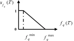
indicates incompatibility with the set, while ‘‘1” means full compatibility [21, 24]. In fuzzy method, a strictly monotonically decreasing and continuous membership function is assigned to each objective. The assigned membership function is 1 at the minimum of objective and 0 at its maximum [21]. The value of the membership function indicates to what extent a solution is satisfying the objectivefq. The decision maker is fully satisfied with objective value of f Xq( )if μf q( ) 1X = and not satisfied at all if
( ) 0
f q X
μ = [21]. There are some types of strictly monotonically decreasing and continuous functions which can be used as membership functions. Here, the linear type has been used for all objectives:
max
min max
max min
min
0 ( )
( )
( ) (
,
, )
1, ( )
max
q q
q q
fq q q q
q q
q q
f X f
f f X
X f f X f
f f
f X f
μ = − ≤ ≤
−
⎧
⎪
⎪
⎨
⎪
⎪
⎩
f
p
(41)
Figure 4 illustrates the graph of this membership function. To determine the membership functions of the criteria, the value of each criterion is calculated separately during the planning horizon. So, individual maximum and minimum values of each objective would be calculated.
Fig. 4. Linear type membership function
By taking the individual minimum and maximum values of each objective function into account, the membership function μf q( )X for each objective function can be determined in a subjective manner. Then, for a multi–objective optimization problem with Q objective functions, the final solution can be found as:
{ }
{
}
,,max min ( ) ; 1,2,...
q
f X q Q
μ = (42)
c) Proposed algorithm
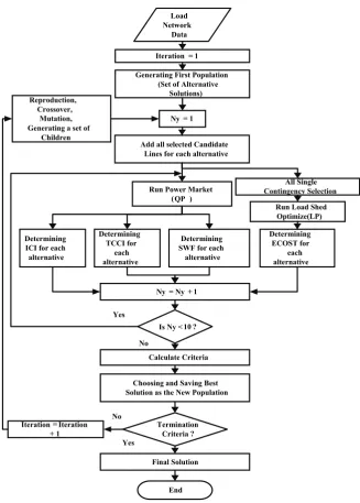
The block diagram of the proposed algorithm is shown in Fig. 5. In Fig. 5, Ny is the number of planning years.
As illustrated in Fig. 5, each alternative will be analyzed to determine its investment cost, congestion cost, social welfare and its ECOST (in all single contingencies) needed for adequate and secure operation. The congestion cost of each alternative is calculated by solving a quadratic optimization problem (Eq. (5)). To calculate the ECOST, a linear optimization problem should be performed for each pre–selected contingency (Eq. (35)).
0 1
( ) q
f x
min
q
f max
q
Fig. 5. Flowchart of the proposed algorithm
5. CASE STUDIES
a) 6–Machine 8–Bus System
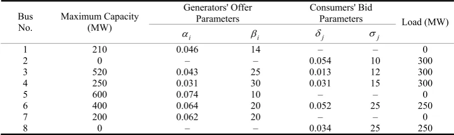
The TEP algorithm was applied to the 6–machine 8–bus test system shown in Fig. 6. Network data for this system can be found in [19–20] and other data are given in the Appendix. The 6–machine 8–bus system consists of six generators at buses 1, 3–7. The total maximum capacity is 2180 MW, and the initial load is 1400 MW, distributed unevenly among the buses which have been increased based on the uncertainties of Table 1. Originally, the system has a total of 11 transmission circuits. Also, the candidate corridors of this study have been selected based on [19–20] to expand the network. In this case study, the four objectives have been considered and all single contingencies have been evaluated. All considered parameters are presented in Table 2. On the other hand, in order to consider load and price uncertainty, two different scenarios have been predicted based on the scenario technique and by the same probability of occurrence
Iteration = 1 Load Network
Data
Generating First Population (Set of Alternative
Solutions)
Choosing and Saving Best Solution as the New Population
Termination Criteria ? Iteration = Iteration
+ 1
Final Solution
End No
Yes
Ny = 1
Add all selected Candidate Lines for each alternative
Run Power Market (QP )
Determining ICI for each alternative
Determining TCCI for
each alternative
Determining SWF for each alternative
Determining ECOST for each alternative
Run Load Shed Optimize (LP)
Ny = Ny + 1
Is Ny < 10 ? Yes
No
Calculate Criteria Reproduction,
Crossover, Mutation, Generating a set of
Children
for the load growth and price growth, which is presented in Table 1 [13].
Fig. 6. Six–machine eight–bus test system.
Table 1. Growth rates for the bid parameters
Years 6–10 1–5 Growth Rate
Scenario N.O
4% 5% Growth rate for demand bid limits (dj,dj)
3% 4% Growth rate of price intercept (βi,σj)
Scenario1
5% 6% Growth rate for demand bid limits (dj,dj)
4% 5% Growth rate of price intercept(βi,σj)
Scenario2
Table 2. Economic and technical parameters
No. Description Quantity
1
Planning 10 horizon years
2
ηsr 4 lines
3
Interest rate %10
4 1200 Construction cost of line $/MW–mile
Population Size =100, Generation=100 Crossover probability=0.9 5
GA parameters
Mutation probability=0.005
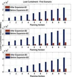
and 8, respectively. As expected, the load curtailment index has increased by network more loading. Figs. 7 and 8, respectively show that with the network expansion, less load curtailment is necessary and the expansion keeps the reliability in an optimized level.
Table 3. Optimal plan based on the first and second scenario
Scenario no Optimal plan
Scenario1 (1–4), (2–3), (8–3), (8–3), (1–7), (1–8), (2–4),(5–8), (6–7) (1–2), (2–3), (2–3), (4–5), (8–3), (8–3), (8–3),
Scenario2 (1–7), (2–4), (2–4), (4–6), (4–6)
Table 4. Objective values of the optimal plan – first scenario
No. Transmission expansion planning indices expansion Before expansion After
1 Investment cost index(m$) 0 1054
2 Total congestion cost index (m$) 11.269 8.211
3 Users' benefit (m$) 68.295 121.891
4 Expected customer interruption Cost (k$/h) 191.208 27.763
Table 5. Objective values of the optimal plan – second scenario
No. Transmission expansion planning indices expansion Before expansion After
1 Investment cost index(m$) 0 915.315
2 Total congestion cost index (m$) 19.199 8.559
3 Users' benefit (m$) 84.130 123.293
4 Expected customer interruption Cost (k$/h) 225.158 32.922
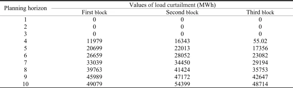
Table 6. Optimal values of the load curtailment – first scenario
Values of load curtailment (MWh)
Third block
Second block
First block
Planning horizon 0 0 0 1 0 0 0 2 0 0 0 3 55.02 16343 11979 4 17356 22013 20699 5 23082 28052 26659 6 29194 34450 33039 7 35753 41424 39763 8 42647 47172 45989 9 48714 54399 49079 10
Table 7. Optimal values of the load curtailment – second scenario
Values of load curtailment (MWh)
Third block
Second block
First block
Fig. 7. The changes of the load curtailment – First scenario
Fig. 8. The changes of the load curtailment – Second scenario
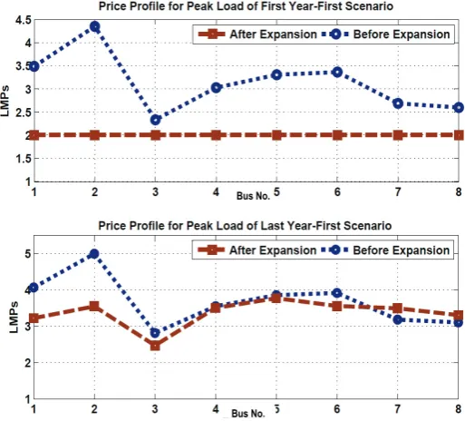
Fig. 9. Price profile for peak load of first and last year– First scenario
Fig. 10. Price profile for peak load of first and last year– Second scenario
b) A real life power system (Iranian Power System)
The proposed method was also applied to a part of the Iranian power system in order to compare the historical expansion plan and the expansion plan developed by the proposed methodology. Fig. 11 shows a simplified northeast part of Iranian national 400–kV transmission grid considered in this case study. Network data for this system (such as investment costs of branches and parameters of bid functions of generator and load levels) can be found in [21]. This part of the Iranian power system network is connected at one point to the main interconnected grid and at another point to the neighboring country, Turkmenistan. A new power plant and a new load bus will be in service at the Shirvan and Kashmar regions, respectively (at the end of planning horizon) and the network should be able to transit a 700 MW wheeling transaction from Turkmenistan to the main interconnected grid.
Bus No.
Bus No.
Bus No. Bus No.
Fig. 11. Northeastern part of Iranian national 400–kV transmission grid
At the planning horizon the total load will be 5766MW and the total installed capacity will be 6150MW (excluding the 700MW wheeling transaction). A generator at the Turkmenistan bus with 700 MW generation at a fixed price (30 $/MWh) and a 700 MW load at the Aliabad bus have been considered for modeling the wheeling transaction. To force the wheeling transaction to 700 MW, minimum and maximum capacities of the generator at Turkmenistan bus are equally defined to 700 MW. It is also assumed that load growth is 8%. All the considered parameters for this network are according to [21]. All the existing lines are considered as candidates. Also, the proposed GA has been tested with the following parameters: population size = 200, generation =100, crossover probability = 0.9, mutation probability = 0.01 [26]. The optimal plan and the extracted costs along with the expansion plan proposed by the Iranian Grid Management Company (IGMC) and [21] are presented in Tables 8 and 9, respectively.
Table 8. Comparison of the proposed algorithm plan, IGMC's practice and ref. [21]
Line IGMC plan Ref. [21] Proposed algorithm plan without users' benefit
L1 0 1 1
L2 1 2 1
L3 1 1 2
L9 1 1 1
L13 1 1 1
L14 1 2 1
L15 0 0 1
L16 0 0 1
L17 1 0 2
Note that the IGMC proposed plan is based on a five–year planning horizon, while in [21] and here in the simulation a ten–year planning horizon has been considered. Table 8 shows that both methods reached almost the same expansion pattern which is the construction and reinforcement of lines L2, L3, L9, L13, and L14. It should be noted that load curtailment values for the proposed algorithm in this study are zero.
Table 9. Comparison of the objectives, IGMC's practice and ref. [21]
Comparison Transmission expansion planning
indices IGMC
plan Ref. [21]
Proposed algorithm plan without users' benefit
Investment cost index (m$) 150.8 185.3 256.702
6. CONCLUSION AND FURTHER WORK
This paper presented a multi–objective model to cope with new challenges introduced by deregulation. The main advantages of the proposed algorithm are: considering requirements of the new deregulated environment, allowing the planner to use a cost–benefit approach instead of the least cost planning procedure, incorporating the static security analysis in the expansion planning which results in a more optimal solution and finally, considering the value – based reliability assessment in the transmission expansion planning process. Also, this method produces a set of optimal solutions in contrast to single objective methods, yielding more flexibility in the planning process. The obtained results from the case studies show the capability of the proposed multi–objective algorithm to handle different planning indices which have different important degrees from the viewpoint of different planners.
There are several ways to improve the proposed algorithm such as using transmission lines along with Flexible AC Transmission Systems (FACTS) devices (such as phase shifter transformers) in the TEP process and considering Virtual Power Plant (VPP) concept (in which the goal of VPP is to allow distributed energy resources to access the energy market) which are under development by the authors.
NOMENCLATURE
b Index of buses.
B Set of all buses.
( )
j j
B d Benefit function of consumer j.
( ) jn e
c t Cost of outage duration te using the Cost function SCDF at sector n of bus j [$/kW].
( )
i i
C g Generation cost of generator i.
( ) j h
CB t Hourly benefit of consumer j.
l
CCI Congestion Cost in line l [$/h].
sr
CL Cost of a circuit that may be added to the corridor s–r.
j
d Active load of consumer j [MW].
j
d ,dj Lower and upper bound for the consumer j. max
jn
d Yearly maximum load demand at bus j.
D Demand vector.
p
D Duration period of pattern p [hour].
e Index of load loss events.
E Set of all load loss events.
l
f Active power flow in line l [MW].
l
f Thermal Capacity in line l [MW].
q
f Individual objective of transmission planning. min
q
f Lower bound for thefq.
max
q
f Upperbound for the fq.
F Active power flow matrix with elementsfsr.
i
g Active generation of generator i [MW].
i
g ,gi Lower and upper bound for the generator i.
G Generation vector.
I Set of all generators.
m
ICI Investment cost index for the plan m.
j Index of consumers.
J Set of all consumers.
l Index of transmission lines.
lmp Locational marginal price [$/MWh].
L Set of all transmission lines.
e
LCC Load Curtailment Cost in state e.
m Index of expansion plans.
n Index of load sectors in each load bus.
N Set of load sectors in each load bus.
p Index of pattern.
P Set of all patterns.
e
sp Probability of state e.
S Node–branch incidence matrix.
( )
i h
SB t Hourly benefit of generator i.
e
t Duration of outage state e.
h
t Index of time [hour].
T Lifetime of transmission lines.
m
T CCI Total congestion cost index for the plan m.
j
T CB Total benefit of consumer j in time T.
i
T SB Total benefit of generator i in time T.
Tot
UB Total Users' Benefit.
jn
w Cost weight factor at sector n of bus j.
x A solution (a combination of corridors to be added to the network).
0
s
y Shunt admittance at bus s.
0
sr
y Initial admittance of branch s–r.
'
e bb
Y The element at the bth row and b' th column in the system susceptance matrix in state e.
i
α ,βi Constants of offer price of generator i.
sr
γ Total susceptance of circuits in corridor s–r.
j
δ ,σj Constants of bid price of consumer j.
p j mCB
Δ Change in hourly benefit due to expansion plan m in pattern p.
p i mSB
Δ Change in hourly benefit due to expansion plan m in pattern p.
mSWF
Δ Change in Social Welfare due to expansion plan m.
Tot mUB
Δ Change in total users' benefit due to expansion plan m.
sr
η Number of new circuits added to the corridor s–r. 0
sr
η Number of initial circuits in corridor s–r.
sr
η Maximum number of new branches which can be existed to the corridor s–r.
θ Phase angle of each bus.
( ) f q x
ν Interest rate.
j
ξ Constant of benefit function of consumer j.
i
π Offer price of generator i [$/MWh].
j
ρ Bid price of consumer j [$/MWh].
sr
τ New circuit admittance of branch s–r.
e jn
χ Amount of curtailed load at sector n bus j in state e.
i
ψ Constant of generation cost of generator i.
Ω Set of all existing and new right–of–ways.
REFERENCES
1. Shayeghi, H., Jalilzadeh, S., Mahdavi, M. & Hadadian, H. (2008). Studying influence of two effective parameters on network losses in transmission expansion planning using DCGA. International Journal of Energy Conversion and Management (Elsevier), Vol. 49, pp. 3017–3024.
2. Latorre, G., Cruz, R. D., Areiza, J. M. & Villegas, A. (2003). Classification of publications and models in transmission expansion planning. IEEE Trans. on Power Systems, Vol.18, pp. 938–946.
3. Wu, F. F., Zheng, F. L. & Wen, F. S. (2006). Transmission investment and expansion planning in a restructured electricity market. International Journal of Energy (Elsevier), Vol. 31, pp. 954–966.
4. Buygi, M. O., Shanechi, H. M., Balzer, G. & Shahidehpour, M. (2003). Transmission planning approaches in restructured power systems. IEEE Bologna power technology conference, Bologna, Italy; June 23–26.
5. Buygi, M. O., Balzer, G., Shanechi, H. M. & Shahidehpour, M. (2004). Market based transmission expansion planning. IEEE Trans. on Power Systems, Vol. 19, No.4, pp. 2060–2067.
6. Buygi, M. O., Shahidehpour, M., Shanechi, H. M. & Balzer, G. (2004). Market based transmission expansion planning: fuzzy risk assessment. In: IEEE international conference on electric utility deregulation, restructuring and power technologies Hong Kong, Vol. 2, pp. 427–432.
7. Buygi, M. O., Shahidehpour, M., Shanechi, H. M. & Balzer, G. (2004). Market based transmission expansion planning: stakeholders’ desires. In: IEEE international conference on electric utility deregulation restructuring and power technologies Hong Kong, Vol. 2, pp. 433–438.
8. De la Torre, S., Conejo, A. J. & Contreras, J. (2008). Transmission expansion planning in electricity markets. IEEE Trans. on Power Systems, Vol. 23, No. 1, pp. 238–248.
9. Kamyab, G. R., Fotuhi–Friuzabad, M. & Rashidinejad, M. (2008). Transmission expansion planning in restructured power systems considering investment cost and (n–1) reliability. Journal of Applied Sciences, Vol. 8, No. 23, pp. 4312–4320.
10. Choi, J., Tran, T., (Rahim) El–Keib, A., Thomas, R., Oh, H. S. & Billinton, R. (2005). A method for transmission system expansion planning considering probabilistic reliability criteria. IEEE Trans. on Power Systems, Vol. 20, No. 3, pp.1606–1615.
11. Braga, S. D. & Saraiva, J. T. (2005). A multiyear dynamic approach for transmission expansion planning and long–term marginal costs computation. IEEE Trans. on Power Systems, Vol. 20, pp. 1631–1639.
12. Xie, M., Zhong, J. & Wu, F. F. (2007). Multiyear transmission expansion planning using ordinal optimization. IEEE Trans. on Power Systems, Vol. 22, pp.1420–1428.
13. Shrestha, G. B. & Fonseka, P. A. J. (2004). Congestion–driven transmission expansion in competitive power markets. IEEE Trans. on Power Systems, Vol. 19, No. 3, pp. 1658–1665.
15. Wangdee, W. (2005). Bulk electric system reliability simulation and application. Ph.D. dissertation, Dept. Elec. Eng., University of Saskatchewan, [Online] Available: http: // library2 .usask. ca /theses /available /etd – 12152005 –133551 /unrestricted /Wijamangdee Phdthesis. pdf.
16. Eliassi, M., Seifi, H. & Haghifam, M. R. (2009). Multi–objective value–based reliability transmission planning using expected interruption cost due to transmission constraint. Electric Power and Energy Conversion Systems (EPECS '09), pp.1–8.
17. Keypour, R., Haghfam, M. R. & Seifi H. (2007). Genetic based long–term transmission expansion planning in competitive electricity markets considering users benefits. Journal of Iranian Association of Electrical and Electronic Engineering (IAEEE), Vol. 4, No. 1, pp. 12–21.
18. Wang, Y., Cheng, H., Wang, C., Hu, Z., Yao, L., Ma, Z. & Zhu, Z. (2008). Pareto optimality–based multi– objective transmission planning considering transmission congestion. International Journal of Electric Power Systems Research (Elsevier), Vol. 78, pp. 1619–1626.
19. Parsa Moghaddam, M., Abdi, H. & Javidi, M. H. (2006). Transmission expansion planning in competitive electricity markets using ACOPF. Power Systems Conference and Exposition (PSCE), pp. 1507–1512.
20. Buygi, M. O. (2004). Transmission expansion planning in deregulated power systems. Ph.D. dissertation, Dept. Elec. Power Systems Institute, Darmstadt University of Technology.
21. Maghouli, P., Hosseini, S. H., Buygi, M. O. & Shahidehpour, M. (2009). A multi–objective framework for transmission expansion planning in deregulated environments. IEEE Trans. on Power Systems, Vol. 24, No. 2, pp.1051–1061.
22. Attaviriyanupap, P. & Yokoyama, A. (2005). Transmission expansion planning in the deregulated power system considering social welfare and reliability criteria. Conference & Exhibition, Asia and Pacific Dalian, China. 23. Xu, Z., Dong, Z. Y. & Wong, K. P. (2006). A hybrid planning method for transmission networks in a
deregulated environment. IEEE Trans. on Power Systems, Vol. 21, No. 2, pp. 925–932.
24. Tran, T., Choi, J., Kwon, J., (Rahim) El–Keib, A. & Watada, J. (2007). Application of fuzzy set theory to transmission system expansion planning. International Symposium on management Engineering (ISME).
25. Albrecht, P. F., et al. (1979). IEEE reliability test system task force of application of probability methods Subcommittee. IEEE Reliability Test System. IEEE Trans. on Power Apparatus and System, Vol. 98, No. 6, pp.2047–2053.
26. Kazemi, A., Ladjevardi, M., Masoum, M.A.S. (2005). Optimal selection of SSSC based damping controller parameters for improving power system dynamic stability using genetic algorithm, Iranian Journal of Science and Technology Transaction B-Engineering (IJST), Vol. 29, No. B1, pp. 1–10.
Appendix The data of the case study network is as follows.
Table A–1. Parameters of offer and bid functions (6 – machine 8 – bus system)
Consumers' Bid Parameters Generators' Offer
Parameters Load(MW)
Table A–2. Candidate lines data (6 – machine 8 – bus system)
No. Type* Line candidate X (P.U) L (km)
1 I 1 2 0.03 230
2 I 1 4 0.03 450
3 I 2 3 0.01 100
4 I 3 4 0.03 350
5 I 4 5 0.03 220
6 I 8 3 0.018 100
7 C 1 7 0.02284 400
8 C 1 8 0.0252 450
9 C 2 4 0.010697 190
10 C 4 6 0.01746 300
11 C 5 8 0.025695 450
12 C 6 7 0.04095 500
*Transmission Lines of the Initial Network (type = I) *Candidate new Transmission Lines (type = C)
Table A–3. Load data (6 – machine 8 – bus system)
Penalty factors ($/kW)
Unit Bus no.
Sector1 Sector2 Sector3
L2 2 8.75 2.5 0.1
L3 3 8.7 2.45 0.15
L4 4 8.65 2.4 0.2
L6 6 8.6 2.35 0.25

![Table 8. Comparison of the proposed algorithm plan, IGMC's practice and ref. [21]](https://thumb-us.123doks.com/thumbv2/123dok_us/21107.2002268/14.595.159.431.61.269/table-comparison-proposed-algorithm-plan-igmc-practice-ref.webp)