Printed in The Islamic Republic of Iran, 2006 © Shiraz University
IMPROVING LOGIC-LEVEL REPRESENTATION OF TAYLOR
EXPANSION DIAGRAM USING ATTRIBUTED EDGES
*P. LOTFI-KAMRAN
**AND Z. NAVABI
Electrical and Computer Engineering Faculty, PARDIS of Engineering Faculties, University of Tehran, Tehran, I. R. of Iran, Email: [email protected]
Abstract– Formal verification of complex digital systems requires a mechanism for efficient representation and manipulation of arithmetic as well as random Boolean functions. Although the Taylor Expansion Diagram can be used effectively to represent arithmetic expressions at the vector level, it is not efficient in the use of memory for representing bit-level logic expressions. In this paper, we present modifications to TED that will improve its ability for logic representation while maintaining its robustness in arithmetic representation. Our experimental results show a 30% reduction in the number of nodes in some benchmarks.
Keywords– Formal verification, Taylor expansion diagram, attributed edge, register transfer level 1. INTRODUCTION
Increasing the size and complexity of digital designs has made it essential to address verification issues in the early stages of the design cycle. This requires verification tools with efficient data structures capable of representing designs at the RT-level.
Most formal verification tools need a design to be converted to a canonical data structure in order for the formal verification algorithms to be used. Several data structures have been proposed to address this need, however none of them, with the exception of TED [1-3], can handle designs at the vector-level. Therefore, formal verification tools today do make use of bit-level representation for capturing a design, and therefore have limitations in processing large designs. On the other hand, a graph-based representation for designs at the RT-level, coupled with efficient algorithms, provides a mechanism for handling large designs. However, TED, which has a good performance in representing vector-level designs, is not good at representing Boolean expressions. Therefore, TED is not efficient for representing designs at the RT-level. In fact, RT-level designs consist of both vector-level and logic-level parts. Many parts of an RT-level design including its controller may be described by Boolean expressions. So, in addition to a good vector-level representation, having a good Boolean function manipulation is essential for an RT-vector-level data structure. The focus of this paper is to introduce Attributed TED, a high-level graph-based representation for the manipulation of RT-level descriptions. This representation is based on TED. This paper addresses the mentioned shortcomings of TED for achieving a better data structure for RT-level representation and formal verification. Experimental results demonstrate that Attributed TED yields better performance than TED using a number of benchmark circuits.
This paper is organized as follows: The following section presents a brief overview of previous works in this area. In Section 3, a brief overview of TED comes. In Section 4, our Attributed TED is introduced. In Section 5, canonicity rules of Attributed TED are mentioned formally and it will be shown that this
∗
Received by the editors November 29, 2005; final revised form April 26, 2006.
∗∗
structure is canonical. In Section 6, some examples are given using Attributed TED. In Section 7, we will show that there are some cases in which Attributed TED is better than TED by a factor of 2. Experimental results are discussed in Section 8, and the conclusion is presented in the last section.
2. PREVIOUS WORKS
Boolean functions are often represented and manipulated by Decision Diagrams (DDs). Ordered Binary Decision Diagrams (OBDDs) [4] are the most commonly used form of decision diagrams in EDA applications [5]. OBDDs are based on a decomposition of Boolean functions commonly called the “Shannon expansion”. A function f can be decomposed in terms of a variable x as:
) 1 ( )
0
( = ∨ ∧ =
∧
=x f x x f x
f (1)
Despite its widespread use, some classes of Boolean functions cannot be represented efficiently by OBDDs [6, 7]. For representing these classes of Boolean functions other decision diagrams are proposed and used. As an example, Ordered Functional Decision Diagrams (OFDDs) [8, 9] are proposed to better represent XOR based logic [10]. OBDDs and their derivations have been successfully used in manipulating gate-level designs, but have limitations in representing arithmetic circuits.
For representing arithmetic circuits, Word Level Decision Diagrams (WLDDs) are proposed. They use decomposition methods similar to the decomposition of Boolean functions, but at the arithmetic-level. MTBDDs [11, 12], EVBDDs [13], BMDs [14], HDDs [15], *BMDs [14], and K*BMDs [16] are examples of WLDDs.
The multi Terminal Binary Decision Diagram (MTBDD) uses a decision graph like a BDD, but allows arbitrary values on the terminal nodes. MTBDDs are very inefficient for representing functions yielding values over a large range.
The Edge Valued Binary Decision Diagram (EVBDD) is the same as MTBDD, but incorporates numeric additive weights on the edges in order to allow greater sharing of sub-graphs. Although EVBDDs improve MTBDDs in many cases, there are still important classes of functions for which they have unacceptable complexity. For example, EVBDDs representation of multiplication x * y grows exponentially.
The Binary Moment Diagram (BMD) is based on a decomposition of functions commonly called the “Moment expansion”. A function f can be decomposed in terms of a variable x as:
x
xf x
f
f = ( =0)+ ∂ (2)
where f∂x = f(x=1)− f(x=0).
Multiplicative Binary Moment Diagram (*BMD) is an extension of BMD to incorporate multiplicative weights on the edges. For some classes of functions, EVBDDs are exponentially more compact than *BMDs, but the reverse can also hold. To obtain the advantages of each, a hybrid form called “Kronecker Multiplicative Binary Moment Diagram” (k*BMD) [16] has been proposed. In k*BMD, each variable has an associated decomposition which can be any one of the three given by Eqs. (1-3). All functions, to be represented, must follow a common variable ordering and every occurrence of a given variable must use the same decomposition.
) 1 ( )) 1 ( ) 0 ( )( 1
( x f f f
f = − − + (3)
With increasing complexity of digital systems, the need for higher level abstraction becomes more evident. TED [1-3] is proposed as an answer to this need. TED can be used for representing functions with an integer domain and integer range. Therefore, in contrast to WLDDs, an arithmetic function should not be broken down into bit-level in order to be represented.
Although TED has good performance in representing arithmetic equations, its weak Boolean function manipulation is its main problem. When a design consists of vector-level and bit-level parts (including Boolean parts), its TED occupies a large amount of memory. One solution is to use different Decision Diagrams for representing different parts of a design. This solution leads to more difficulties in the verification process. Also using two or more different decision diagrams makes it hard, almost impossible to check the equivalency of two designs, since the equivalency of two designs does not mean that each of their parts is necessarily equivalent.
The aim of this paper is to improve logic representation of TED. This paper provides a unique representation for better representing typical algebraic equations as well as Boolean functions.
3. AN OVERVIEW OF TED
TED is a graph-based representation which uses the Taylor series as its decomposition method [1-3]. The Taylor series of a real differentiable function f(x) around x=0 are:
L + ′′′ +
′′ +
′ +
= (0)
! 3 1 ) 0 ( ! 2 1 ) 0 ( ) 0 ( )
(x f xf x2f x3f
f (4)
where f′(0), f ′′(0), and f ′′′(0) are first, second, and third derivatives of function f around x=0 respectively. The decomposition will be performed recursively using Eq. (4).
Every node of a TED representation has a label that indicates its associated variable. As in most canonical decision diagrams, e.g., OBDD, the variables of TED are ordered. The function of a node is determined by the Taylor series expansions, according to Eq. (4). The out-degree of a node depends on the order of the associated variable of that node. The out-degree of a terminal node is 0.
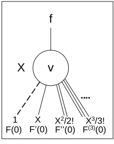
Fig. 1. Decomposition in TED
Figure 1 shows TED decomposition of function f for variablex. In this paper, we refer to the k-th derivative of a function rooted at a node as k-child of that node: f(x=0) is the 0-child, f′(x=0) is the 1-child, f ′′(x=0) is the 2-child, etc. We also refer to the corresponding edges as 0-edge (dotted), 1-edge (solid), 2-edge (double), etc. From the Taylor expansion, it is evident that each edge has an implicit multiplicative factor, i.e., x0 for the 0-edge, x1 for the 1-edge, x2/2 for the 2-edge, etc. In addition, each edge in a TED has a multiplicative weight, which is computed from the Taylor expansions. Figure 2 shows TED representation of x2+y.
X
1 X X2/2! X3/3!
f
F(0) F’(0) F’’(0) F(3)(0)
x F = x2+y
F(x= 0) =
y
F’( x= 0) = 0
F
’’(
x
=
0
)
=
2
y
1 0
2 F = x2+y
F’ = 2x F’’ = 2
Fig. 2. TED decomposition of x2+y
It has been proven that with a special restriction on the order of variables, TED becomes a canonical representation. For functions typically encountered in RTL specifications (e.g., x – y, x + y, x * y and xk for arbitrary k, etc.), TED is linear in the number of variables. TED can also represent functions containing both algebraic and Boolean expressions. To represent Boolean expressions, the following formulae should be used [1-3]:
NOT(x) = a′ = 1 – a (5)
AND(a, b) = a ∧ b = a * b (6)
OR(a, b) = a ∨ b = a + b – a * b= a(1 – b)+ b (7)
4. ATTRIBUTED TED
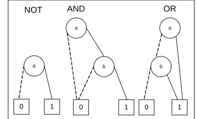
Representing Boolean functions is the main problem of TED. This means that the TED representation of a Boolean function has a larger size when compared with BDD representation of the same function. Consider the TED representation of three basic Boolean functions (AND, OR, NOT) in Fig. 3 and BDD representation of these functions in Fig. 4.
a
1 1
b
0 1
a
b
0 1
a
NOT(1-a) AND(a*b) OR(a+b-a*b)
b
-1
-1 +1
0 0
1
1 0
1
1 1
1
a
0 1
b
0 1 a
b
0 1 a
NOT AND OR
Fig. 3. TED representation of basic Boolean functions Fig. 4. BDD representation of basic Boolean functions As shown, NOT and AND functions are presented with minimal nodes, but the OR function has some extra nodes in comparison with its BDD. Since the OR function is one of the basic Boolean functions, extra nodes would be produced during the process of TED construction for Boolean functions, and the size of TED increases drastically. So improving the TED representation of the OR function would reduce the size of TED representation of Boolean functions.
As explained, the TED of OR function is constructed according to Eq. (7), where ‘a’ and ‘b’ are two valued integer variables (0 and 1). If we consider the ‘a’ variable as root, then two edges are originated from it:
• 0-child, which is equal to ‘b’
As ‘a’ and ‘b’ are two valued variables (0 and 1), ‘1−b’ function logically is the complement of ‘b’. This property can be used for graph reduction. Indeed, the sub-graph of ‘b’ representation can be shared between 0-child and 1-child of the root node. This can be done by adding an attribute to the structure of the edges. This attribute is used to show the complement of the following node. For example, the TED representation of the OR function is converted to the graph shown in Fig. 5.
b
0 1
a
b b
0 1
a
0
0 1 1
1 1
0 1
1 1
Fig. 5. Attributed TED representation of OR function
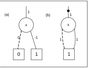
If an edge points to a sub-function which should be complemented, only the attribute of the edge is set to indicate this. These edges are called attributed edges. This change should be done in such a way that the Attributed TED remains canonical as the original TED. Although attributed edges have the advantage shown here, their use must be restricted in order for the resulting structure to be canonical. We will show how freedom in the use of attributed edges can cause two equivalent expressions to be represented differently, by use of the example of expressions (8) and (9).
-x (8)
1 – (x + 1) (9)
It is evident that expressions (8) and (9) are equal, but the TEDs with attributed edges of these two equations are different. For the former, the TED of “–x” is created, but for the latter, the TED of “x + 1” is created and then the attribute of the created TED is set true. As shown in Fig. 6, the two TEDs are not the same.
x
0 1
x
1
-1
(a) (b)
0 1
1 1
1
Fig. 6. a) TED of expressions (8), b) TED of expressions (9)
In the next section, some rules are introduced for restricting the use of attributed edges and for preserving the canonicity of the Attributed TED. It will be shown that canonical Attributed TED can reduce the size of certain Boolean functions by a factor of 2.
5. CANONICITY RULES
Attributed TED remains canonical, if we follow rules discussed below.
2. If a 0-edge is attributed and its weight is 1, we remove the attribute of the 0-edge, negate the value of weights of other neighboring edges, and instead attribute the incoming edge of that node.
Theorem 1: The above rules do not change the function corresponding to TED.
Proof: by Rule 1, we mean that a 1-terminal is replaced with a 0-terminal, and an attribute in the edges pointing to it is set true to perform complementing. It is obvious that these modifications do not change the function corresponding to the resulting TED.
Rule 2 needs more explanations. For complementing a function named f(x), 1 – f(x) should be constructed (i.e., Eq. (5)). The Taylor series of 1 – f(x) is as follows:
L
− −
′′ −
′ − − =
− (0)
! 3 1 ) 0 ( ! 2 1 ) 0 ( ) 0 ( 1 ) (
1 f x f xf x2f x3f(3) (10)
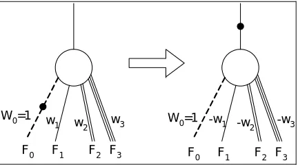
By comparing Eq. (4) and (10), it is obvious that for calculating the complement of f(x), we should complement its 0-edge (i.e., f(0)) to come up with 1 – f(0). Furthermore, we should negate the weights of all other edges of this function. By Rule 2, we mean that attributed edges should not be used in the 0-edges of the Attributed TED with weight 1. This is done so that all required attributes move as far up in the Attributed TED as possible. This procedure is exemplified in Fig. 7 and discussed as follows: If the 0-edge of a node has its attribute true and its weight is 1, it is complemented (i.e., the precedence of attribute is higher than weight, so only if weight is 1, the function of that edge is complemented), we de-complement the function of the node by resetting the attribute of the 0-edge and negating the weights of other edges, and instead set the attribute of the incoming edge of that node itself.
W0=1 w
1 w2 w3 W0=1 -w1 -w2 -w3
F0 F1 F2 F3 F
0 F1 F2 F3
Fig. 7. Exemplifying the procedure of Rule 2 Theorem 2:Attributed TED made by Rules 1 and 2 is canonical.
Proof: The proof of this theorem is conceptually straightforward. The proof proceeds by induction on the size of the argument set of a function (f).
If the size of the argument set is 0, f must be a constant function. This constant function has a terminal (T) and an edge with a weight (W) and an attribute (A). Let’s say that this constant function is represented by two such graphs, G1(T1, W1, A1) and G2(T2, W2, A2). Since we have used Rule 1, a terminal value can only be 0. So, the two graphs cannot be different in their terminal values (T1 = T2). So, if G1 and G2 are different, either W1 and W2 or A1 and A2 are different. W1 and W2 cannot be different because both graphs originated from the same TED and Rule 1 only changes attributes and not the weights. Note that because f(x) is a constant, only Rule 1 can be applied to it. On the other hand, if G1 and G2 are to be different, A1 and A2 must be different. This would result in two different functions, which is contradictory to our original assumption of having only one function.
assumption we will show that representation of functions of k variables are also canonical. Note that function f is represented in Attributed TED by a node and several child functions of k-1 variables.
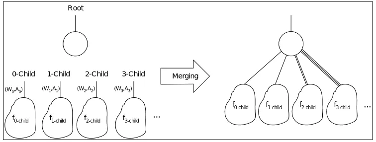
Now if the Attributed TED representation of f is not canonical, there must be two different G1 and G2 representations of it. According to our earlier assumption, the representations of all functions of the root’s children are independently canonical. Figure 8 shows this decomposition. Merging functions of the root’s children into the root forms the complete representation of f. In this formation, individual nodes of functions of the root’s children remain unchanged, and the only possible change will be in the weights or attributes of the edges that connect the children to the root.
The weights of G1 and G2Attributed TED graphs of function f cannot be different, since these weights are the greater common divisor of all weights of edges that connect children to the root. Similarly, based on Rule 2, attributes affect all edges of G1 and G2 in the same way and cannot make these graphs different. This means that the only possible difference between G1 and G2 is in their root’s label, which would make two different functions if they were different. Since this contradicts our main assumption, G1 and G2 must be the same.
f0-child f1-child f2-child f3-child (W0,A0)
0-Child
(W1,A1) (W2,A2) (W3,A3)
1-Child 2-Child 3-Child
... Root
Merging
f0-child f1-child f2-child f3-child ...
Fig. 8. Merging Root’s children into the Root
6. EXAMPLES
In this section, applications of the above rules are presented by use of several examples. Consider the TED representation of the OR function in Fig. 3. The first step towards attributed representation is replacing 1 -terminals by 0-terminals. According to Rule 1 attributes of the edges which are pointing to terminals 1 should be set. This step is shown in Fig. 9b.
a
b b
0 1 -1
a
b b
0 -1
a
b b
0 +1
a
b
0
(a) (b) (c) (d)
0 1 1
1 1
0 1 1 1 1
1 1 0
1 1
0 1 1 1
Fig. 9. Steps of applying Rules 1 and 2 to the TED representation of OR function
redundant nodes. As shown in Fig. 9c, two b nodes are exactly similar and they can be merged. The result and the final Attributed TED of the OR function is shown in Fig. 9d.
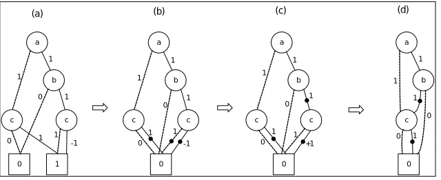
The efficiency of this method would be shown when the TEDs of more complex Boolean functions are compared with the attributed ones. As an example, consider functionF =(a∧b)∨c. The TED of this function is shown in Fig. 10a.
This graph can be reduced by applying the previous rules. Figure 10b shows the result graph after applying Rule 1 and Fig. 10c shows the result graph after applying Rule 2. As shown, some redundant nodes are generated in the graph after these conversions. The final step is merging the redundant nodes. Figure 10d shows the final Attributed TED representation ofF=(a∧b)∨c.
a b c c 0 1 -1 a b c c 0 -1 a b c c 0 +1 a b c 0
(a) (b) (c) (d)
0 0 1 1 1 1 1 1 1 1 0 0
1 1 1
0 1 0 1 1 1 1 1 0 1 0 1
Fig. 10. Steps of applying Rules 1 and 2 to TED representation of F=(a∧b)∨c
By comparing this graph and the initial TED representation graph, a gain of 25 percent is evident.
7. CASE STUDY
Lemma 1: The total number of nodes for representing i n
i x OR
1
= (OR of n different Boolean variables) by the original TED is computed from the following recursive equation:
2 ) 1 ( )
(n =TotalNumNodes n− + des
TotalNumNo TED TED
Proof: For representing i n
i x OR
1
= by TED, the following arithmetic equation should be constructed:
n n n n n x x x x x x x x x x x x x x x x x x x x f L L L L L L 3 2 1 3 2 1 1 3 2 1 3 1 2 1 2 1 + − + + − − − − − − − + + + = −
To represent this equation by TED, we need a root node that is associated with variable x1. The root’s
children are ( 0)
1 =
x
f (0-child) and ( 1 0)
1 = x dx df (1-child). n n n n n x x x x x x x x x x x x x x x x x x x f L L L L L L 3 2 4 3 2 1 4 3 2 4 2 3 2 2 ) 0 ( 1 + − + + − − − − − − − + + = = − n n n n n x x x x x x x x x x x x x x x x x x x dx df L L L L L L 3 2 4 3 2 1 4 3 2 4 2 3 2 2 1 1 1 ) 0 ( − + − − + + + + + + + − − − = = −
It is evident that ( 0)
1 =
x
f is i
n
i x OR
2
= , therefore it needs TotalNumNodesTED(n−1) TED nodes for its
construction. On the other hand, ( 1 0)
1 =
x dx
df
is i
n i x OR 2 1 =
− or ( )
2 i n
i x OR NOT
an associated variable being x2 for representing this function. The children of this new node are
) 0 , 0
( 1 2
1 = = x x dx df
(0-child) and ( 1 0, 2 0)
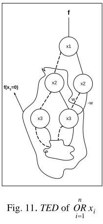
2 1 = = x x dx dx df (1-child). n n n n n x x x x x x x x x x x x x x x x x x dx df L L L L L L 4 3 5 4 3 1 3 5 3 4 3 3 2 1 1 1 ) 0 , 0 ( − + − − + + + + + + − − − = = = − n n n n n x x x x x x x x x x x x x x x x x x dx dx df L L L L L L 4 3 5 4 3 1 3 5 3 4 3 3 2 1 2 1 1 ) 0 , 0 ( + − + + − − − − − − + + + − = = = −
By comparing the above equations, we conclude:
) 0 , 0
( 1 2
1 = = x x dx df = i n i x OR 3 1 = − = ( ) 3 i n i x Or NOT =
This function is already constructed during generation of ( 0)
1 =
x
f . Also it is clear
that ( 1 0, 2 0)
2 1 = = x x dx dx df
is negation of the ( 1 0, 2 0)
1 = = x x dx df
(if the weight of ( 1 0, 2 0)
2 1 = = x x dx dx df
is w,
the weight of ( 1 0, 2 0)
1 = = x x dx df
is -w). So, by connecting an edge with negative weight to the node which
represents ( 1 0, 2 0)
1 = = x x dx df
, this function is constructed.
w -w
f(x1=0)
f
x2 x1
x2
x3 x3
Fig. 11
.
TED of i ni x OR
1 =
So, the i n
i x OR
1
= function is represented by:
2 ) 1 ( )
(n =TotalNumNodes n− + des
TotalNumNo TED TED
TED nodes.
Lemma 2: The total number of nodes for representing i n
i x OR
1
= (OR of n different Boolean variables) by the Attributed TED is computed from the following recursive equation:
1 ) 1 ( )
(n =TotalNumNodes n− +
des TotalNumNo
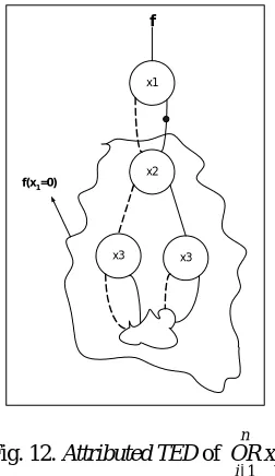
Proof: the proof is the same as Lemma 1, but the 1-edge of the root points to the ( 0)
1 =
x
f (i.e., 0-child),
while having its attribute true to indicate that this function is complemented.
Therefore, for construction of i n
i x OR
1 =
1 ) 1 ( )
(n =TotalNumNodes n− + des
TotalNumNo
ATED ATED
Attributed TED node is needed.
f(x1=0)
x3 x2
x3 x1
f
Fig. 12. Attributed TED of i n
i x OR
1 =
Theorem3: In representing a chain of OR gates, Attributed TED is better than the original TED by a factor of 2. This can be deduced from Lemmas 1 and 2.
8. EXPERIMENTAL RESULTS
In this section, we describe experimental results that have been carried out on a PC Pentium 4 with 1 GByte of memory. All runtimes are given in CPU seconds. BDD, BMD, TED, and Attributed TED packages are implemented by the authors with Visual C++ v6.
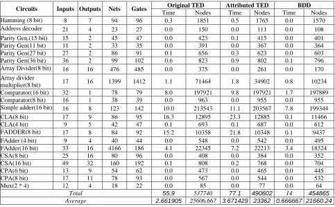
Table 1 provides a summary of the results obtained for several gate-level benchmark circuits. These circuits have BDDs with at least 50 nodes. The column labeled BDD shows the result of converting these circuits to BDD, while sub-columns show the number of BDD nodes and time of conversion. TED and Attributed TED columns show the same parameters for TED and Attributed TED diagrams. All diagrams are built based on the same variable orderings.
The number of nodes in the Attributed TED is always less than that of the original TED. TED is better than Attributed TED in terms of time of conversion. This is due to the complexity of handling the edge’s attribute in the Attributed TED.
The circuits selected for experiments are the real world arithmetic units. Table 1 shows that on average, we have a 9% improvement when using Attributed TED as compared with TED. However, Attributed TED has about 7% more nodes than BDD.
Table 1. TED, Attributed TED, and BDD construction results for various circuits
Original TED Attributed TED BDD Circuits Inputs Outputs Nets Gates
Time Nodes Time Nodes Time Nodes
Hamming (8 bit) 8 7 94 96 0.3 1851 0.5 1765 0.0 1570
Address decoder 21 4 23 27 0.0 150 0.0 111 0.0 108
Parity Gen.(15 bit) 15 2 45 47 0.0 423 0.1 415 0.0 401
Parity Gen(11 bit) 11 2 33 35 0.0 391 0.0 367 0.0 364
Parity Gen(27 bit) 27 2 86 91 0.1 656 0.3 623 0.0 603
Parity Gen(36 bit) 36 2 99 102 0.6 823 0.9 802 0.1 796
Array Divider(8 bit) 16 16 476 485 0.0 375 0.0 261 0.0 170
Array divider
multiplier(8 bit) 17 16 1399 1412 1.1 71464 1.8 34902 0.8 10234
Comparator(16 bit) 32 1 78 79 8.0 197921 9.8 197921 1.7 197889
Comparator(8 bit) 16 1 38 39 0.0 963 0.0 955 0.0 955
Simple adder(16 bit) 16 8 123 142 10.0 213543 11.1 203567 7.8 199344
CLA(8 bit) 17 9 86 95 16.3 12895 23.3 12885 0.1 11466
CLA(4 bit) 9 5 42 47 0.1 693 0.1 687 0.0 612
FADDER(8 bit) 17 8 84 92 15.2 10358 21.8 10348 0.1 9437
FAdder (4 bit) 9 4 40 44 0.0 548 0.0 542 0.0 495
FAdder(16 bit) 33 16 4166 186 4.1 22345 7.2 22213 3.4 18324
CSA(8 bit) 25 16 80 96 0.0 408 0.0 384 0.0 352
CSA(16 bit) 49 32 160 192 0.1 808 0.2 768 0.0 704
CPA(6 bit) 13 9 54 62 0.0 473 0.0 465 0.0 445
CPA(8 bit) 17 11 78 93 0.0 567 0.0 544 0.0 532
Mux(2 * 4) 12 4 18 22 0.0 85 0.0 77 0.0 64
Total 55.9 537740 77.1 490602 14 454865
Average 2.661905 25606.667 3.671429 23362 0.666667 21660.24
Figure 13 shows a chart for the number of nodes in three structures. As shown, charts corresponding to Attributed TED nodes and BDD nodes are close, but for TED, it is significantly different.
The time spent for circuit conversion of different structures is shown in the chart of Fig. 14. More time is spent for the conversion of Attributed TED when compared with TED and BDD. This is because of the high complexity of algorithms in this structure.
Different Diagrams
0 50000 100000 150000 200000 250000
1 4 7 10 13 16 19 22
Circuit No.
N
u
m
b
e
r of
N
o
de
s
Original TED
BDD Improved TED
Conversion Time
0 5 10 15 20 25
1 4 7 10 13 16 19 22
Circuit No.
Ti
m
e BDD
Improved TED
Original TED
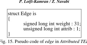
Fig. 13. Number of nodes in different structures Fig. 14. Time of conversion in different structures For implementing attributed edges in Attributed TED, we have used bit-fields in the C++. A structure like that of the Fig. 15 pseudo-code is used.
struct Edge is {
signed long int weight : 31; unsigned long int attrib : 1; }
Fig. 15. Pseudo code of edge in Attributed TED
In the last series of experiments, we compared the capabilities of BMD, TED and Attributed TED for representing RT-level benchmarks. Table 2 provides a summary of the results obtained for these benchmark circuits. Of the ten benchmarks, Paulin is a differential equation solver, described in detail in [17]. Chain_mult is based on the circuit given in [18]. The SimpleCPU is a processor and described in [19]. The SimpleRTL is described in [20]. The 5th Order Elliptical filter is described in detail in [21]. The Avenhause filer is described in [22]. All other benchmarks are described in [23]. All diagrams are built based on the same variable orderings.
Attributed TED is better than TED in terms of the number of nodes. However, its conversion time is almost the same as TED’s. This is due to the fact that logic-level representation of Attributed TED is better than TED’s. In addition, because of the smaller number of nodes, the time of conversion of TED’s and Attributed TED’s are almost the same (smaller number of nodes compensate the higher complexity of algorithms of Attributed TED). Also, Attributed TED and TED are better than BMD in terms of the number of nodes and time of conversion. Table 2 proves that Attributed TED is a good candidate for representing designs at the RT-level.
Table 2.Comparison among BMD, TED, and Attributed TED through several RT-level benchmarks
BMD TED Attributed TED
Benchmark
Nodes Time Nodes Time Nodes Time
SimpleCPU 687 31 407 15 381 15
Chain_mult 282 15 114 15 98 16
Paulin 1017 62 380 31 367 32
SimpleRTL 334 16 159 2 150 3
Avenhaus Filter 1093 46 372 15 351 17
3rdOrder IIR 1129 62 380 15 362 15
4 Point DCT 1332 62 406 16 391 16
5thOrder Elliptical Filter 4718 313 2240 141 2103 145 6 Tap Wavelet Filter 4363 219 1171 62 1023 64
6th Order FIR 3737 219 727 31 635 32
9. CONCLUSION
In this paper, Attributed TED has been proposed. An attribute has been added to each edge of our new Attributed TED. When an edge needs to point to a complemented part, it simply points to a non-complemented one and sets its attribute to show this. This way, only non-non-complemented functions and sub-functions should be constructed directly.
a better solution for representing designs containing both gate-level (Boolean expressions) and vector-level (arithmetic equations) parts than TED.
REFERENCES
1. Kalla, P., Ciesielski, M., Boutillon, E. & Martin, E. (2002). High-level design verification using Taylor Expansion Diagrams: first results. High-Level Design Validation and Test Workshop, 13-17.
2. Ciesielski, M., Kalla, P., Zeng, Z. & Rouzeyre, B. (2001). Taylor expansion diagrams: a new representation for RTL verification. High-Level Design Validation and Test Workshop, Pages 70-75.
3. Ciesielski, M. J., Kalla, P., Zeng, Z. & Rouzeyre, B. (2002). Taylor expansion diagrams: a compact, canonical representation with applications to symbolic verification. Design, Automation and Test in Europe, 285-289. 4. Bryant, R. E. (1986). Graph-based algorithms for Boolean function manipulation. IEEE Transactions on
Computers, 35, 677-691.
5. Bryant, R. E. (1992). Symbolic Boolean manipulation with ordered binary decision diagrams. ACM Computing Surveys, 24, 293-318.
6. Becker, B., Drechsler, R. & Werchner, R. (1995). On the relation between BDD’s and FDD’s. Information Computing, 123, 185-197.
7. Rudell, R. (1993). Dynamic variable ordering for ordered binary decision diagrams. International Conference on CAD, 42-47.
8. Drechsler, R., Theobald, M. & Becker, B. (1994). Fast OFDD based minimization of fixed polarity Reed-Muller expressions. European Design Automation Conference, 2-7.
9. Kebschull, U., Schubert, E. & Rosenstiel, W. (1992). Multilevel logic synthesis based on functional decision diagrams. European Design Automation Conference, 43-47.
10.Drechsler, R. & Becker, B. (1997). Sympathy: Fast exact minimization of fixed polarity Reed-Muller expressions for symmetric functions. IEEE Transactions on CAD, 16, 1-5.
11.Clarke, E. M., McMillan, K. L., Zhao, X., Fujita, M. & Yang, J. (1993). Spectral Transforms for Large Boolean Functions with Applications to Technology Mapping. Design Automation Conference, 54-60.
12.Bahar, R. I., Frohm, E. A., Gaona, C. M., Hachtel, G. D., Macii, E., Pardo, A. & Somenzi, F. (1993). Algebraic decision diagrams and their applications. International Conference on CAD, 188-191.
13.Lai, Y. T., Pedram, M. & Vrudhula, S. B. K. (1996). Formal verification using edge-valued binary decision diagrams. IEEE Transactions on Computers, 45, 247-255.
14.Bryant, R. E. & Chen, Y. A. (1995). Verification of arithmetic circuits with binary moment diagrams. Design Automation Conference, 535-541.
15.Clarke, E. M., Fujita, M. & Zhao, X. (1995). Hybrid decision diagrams-overcoming the limitation of MTBDDs and BMDs. International Conference on CAD, 159-163.
16.Drechsler, R., Becker, B. & Ruppertz, S. (1997). The K*BMD: A verification data structure. IEEE Design & Test of Computers, 14, 51-59.
17.Ghosh, I., Raghunathan, A. & Jha, N. K. (1998). A design-for-testability technique for register-transfer level circuits using control/data flow extraction. IEEE Transactions on CAD, 17, 706-723.
18.Ravi, S., Ghosh, I., Roy, R. K. & Dey, S. (1998). Controller resynthesis for testability enhancement of RTL controller/data path circuits. International Conference on VLSI Design, 193-198.
19.Lotfi-Kamran, P., Hosseinabady, M., Shojaei, H., Massoumi, M. & Navabi, Z. (2005). TED+: A data structure for microprocessor verification. Asia and South Pacific Design Automation Conference, 567-572.
20.Ravi, S., Lakshminarayana, G. & Jha, N. K. (2001). TAO: regular expression-based register-transfer level testability analysis and optimization. IEEE Transactions on VLSI, 9, 824-832.
22.Hong, I. & Potkonjak, M. (1998). Techniques for functional test pattern execution. Asia and South Pacific Design Automation Conference, 283-288.
23.Kin, H. B. (1999). High-level synthesis and implementation of built-In self-testable data path intensive circuit. Ph.D. dissertation, Department of Electrical and Computer Engineering, Virginia Polytechnic Institute and State University, Blacksburg, Virginia.
24.Minato, S., Ishiura, N. & Yajima, S. (1990). Shared binary decision diagram with attributed edges for efficient Boolean function manipulation. Design Automation Conference, 52-57.