Two-Aircraft optimal control problem. The in-flight noise reduction*,, **

(1)

Fédération Denis Poisson (Orléans-Tours) et E. Trélat (UPMC), Editors

TWO-AIRCRAFT OPTIMAL CONTROL PROBLEM. THE IN-FLIGHT NOISE

REDUCTION

∗,∗∗

Fulgence Nahayo

1

, Mounir Haddou

2

, Salah Khardi

3

, Mahmoud Hamadiche

4

and Jean Ndimubandi

5

Abstract. The aim of this paper is to present and solve a mathematical model of a two-aircraft optimal control problem reducing the noise on the ground during the approach. The mathematical modelization of this problem is a non-convex optimal control governed by ordinary non-linear dif-ferential equations. To solve this problem, A direct method and a Runge-Kutta RK4 discretization schema are used. This discretization schema is chosed because it is a sufficiently high order and it does-not require computation of the partial derivatives of the aircraft dynamic. The Nonlinear Interior point Trust Region Optimization solver KNITRO is applied. A large set of numerical experiments is presented. The obtained results give feasible trajectories with a significant noise reduction.

Introduction

In this work, a theoretical model of noise optimization is developped while maintaining a reliable evolution of the flight procedures of two commercial aircraft on approach. In particular, this work is focused on aircraft coupling noise levels and energetic consumption. These two-aircraft are supposed to land successively on one runway without conflict [20].

The model considered here is convex and linear optimal control problem leading to a system of linear ordinary differential equations [6]. The aircraft dynamic is described by a three dimensional set of non-linear ordinary differential equations subjected to state and control constraints. The functional to be minimized describes the overall levels of noise collected on the ground, emitted by the two mentioned aircraft. The formulation of the problem takes into account several kinds of constraints such as aircraft stability, performance and flight safety. The Nonlinear Interior point Trust Region Optimization solver ’KNITRO’ [21] is used to solve the obtained algebric non-linear system of equation implemented by A Modeling Language for Mathematical Programming ’AMPL’ [9, 17].

∗_{This work is supported by the Agence Universitaire de la Francophonie and the French Institute of Science and Technology} for Transport, Development and Networks - Transport and Environment Laboratory ”IFSTTAR-LTE”, Lyon - France. ∗∗_{Authors would like also to thank La R´}_{egion Rhˆ}_{ones-Alpes for the support given in Cluster de Recherche: Transport, Territoire} et Soci´et´e framework.

1

Infomaths, University Claude Bernard of Lyon 1 - LTE-IFSTTAR - University of Burundi,E-Mail: [email protected]

2

INSA-IRMAR, UMR-CNRS 6625, Rennes - France.

3

LTE, The French Institute of Science and Technology for Transport, Development and Networks, Lyon - France

4

LMFA,University Claude Bernard of Lyon 1, France

5

Mathematics departement, University of Burundi, Bujumbura - Burundi

c

EDP Sciences, SMAI 2012

(2)

The two-aircraft flight dynamic, the noise levels, the constraints, the mathematical basic equations of the two-aircraft acoustic optimal control problem and the discretization scheme are presented in sections 2 and 3 while the numerical experiments are presented in the last section.

1. _{Mathematical description of the basic equations}

1.1. Aircraft dynamic equations

The equations of 3D-motion of each aircraftAi, i∈ {1,2} read [3, 4]:

                                                                   ˙

mi =−2.01×10−5

(Φ−µi−Kiηc)

√

Θ √

5ηn(1+ηtfiλ)

r

Gi+0.2Mi2 ηdi ηtfi

λ−(1−λ)Mi

P0δxiρ_ρ0i(1−Mi+

M2

i

2 ),

˙ Vai =

1

mi[−migsinγai−

1

2ρiSV

2

aiCDi+ (cosαaicosβai+sinβai+sinαaicosβai)Fxi

+CSRiP0δxi

ρi

ρ0(1−Mi+

M2

i

2 )ui−mi∆Aiu],

˙ βai =

1

miVai[migcosγaisinµai+

1

2ρiSVa2iCyi+ [−cosαaisinβai+cosβai−sinαaisinβai]Fyi,

+CSRiP0δxi

ρi

ρ0(1−Mi+

M2

i

2 )vi−mi∆Aiv],

˙ αai =

1

miVaicosβai[migcosγaicosµai−

1

2ρiSVa2iCLi+ [−sinαai+cosαai]Fzi

+CSRiP0δxi

ρi

ρ0(1−Mi+

M2

i

2 )wi−mi∆Aiw],

˙

pi = _ACC₋_E2{riqi(B−C)−Epiqi+1

2ρiSlV

2 aiCli+

P2

j=1Fj[ybMijcosβmijsinαmij−z

b

Mijsinβmij]},

+_ACE₋_E2{piqi(A−B)−Eriqi+

1

2ρiSlVa2iCni+

P2

j=1Fj[xbMijsinβmij−y

b

Mijcosβmijcosαmij]},

˙

qi = _B1{−ripi(A−C)−E(p2i −ri2) +12ρiSlV 2 aiCmi

+P2

j=1Fj[zMbijcosβmijcosαmij−x

b

Mijcosβmijsinαmij]},

˙

ri = _ACE₋_E2{riqi(B−C) +Epiqi+

1

2ρiSlV

2 aiCli+

P2

j=1Fj[ybMijcosβmijsinαmij−z

b

Mijsinβmij]},

+ A

AC−E2{p_iq_i(A−B)−Er_iq_i+1

2ρiSlV

2 aiCni+

P2

j=1Fj[xbMijsinβmij−y

b

Mijcosβmijcosαmij]},

˙

XGi =Vaicosγaicosχai+uw,Y˙Gi =Vaicosγaisinχai+vw,Z˙Gi=−Vaisinγai+ww,

˙

φi =pi+qisinφitanθi+ricosφitanθi,θ˙i=qicosφi−risinφi,ψ˙i=sinφ_cosθ_iiqi+cosφ_cosθ_iiri,

(1) where j ∈ {1,2} stands for the first and second engine of each aircraft i, the expressions A = Ixx, B =

Iyy, C =Izz, E =Ixz are the inertia moments of the aircraft,ρi is the air density, S is the aircraft reference

area, l is the aircraft reference length, g is the acceleration due to gravity, CDi = CD0+kC

2

Li is the drag

coefficient, Cyi =Cyββ+Cyppl_V +Cyrrl_V +CY δlδli+CY δnδni is the lateral forces coefficient, CLi=CLα(αa−

αa0) +CLδmδmi+CLMMi+CLq

qb al

V is the lift coefficient,Cli=Clββ+Clp pl V +Clr

rl

V +Clδlδli+Clδnδniis the

rolling moment coefficient, Cmi =Cm0+Cmα(α−α0) +Cmδmδmi is the pitching moment coefficient, Cni=

Cnββ+Cnppl_V +Cnr_Vrl+Cnδlδli+Cnδnδniis the yawing moment coefficient, (x

b

Mij, xbMij, xbMij) is the position of

the engine in the body frame,P0is the full thrust,ρ0is the atmospheric density at the ground,F = (Fxi, Fyi, Fzi)

is the propulsive force, Vai = (ui, vi, wi) is the aerodynamic speed, (∆Aiu,∆Aiv,∆Aiw) is the complementary

acceleration, (uw, vw, ww) is the wind velocity,βmijis the yaw setting of the engine andαmijis the pitch setting

of the engine. The mass change is reflected in the aircraft fuel consumption as described by E. Torenbeek [19]

where the specific consumption isCSRi = 2.01×10−

5 (Φ−µi−Kiηc)

√

Θ √

5ηn(1+ηtfiλ)

r

Gi+0.2Mi2 ηdi ηtfi

λ−(1−λ)Mi

with the generating

functionGi = (Φ−K_η_ci)(1− 1.01 η

ν−1

ν

i (Ki+µi)(1−Φ_ηcηtKi )

), Ki =µi(ǫ

ν−1

ν

c −1), µi = 1 + ν−₂1Mi2. The nomenclature of

engine performance variables are given by Gi the gas generator power function, G0 the gas generator power

function (static, sea level), K the temperature function of compression process,Mithe flight Mach number, T4

the turbine Entry total Temperature, T0 the ambient temperature at sea level, T the flight temperature, while the nomenclature of engines yields isηc= 0.85 the isentropic compressor efficiency,ηdi = 1−1.3(

0.05

Re

1 5)

2₍0.5

Mi)

2L

(3)

the isentropic fan intake duct efficiency,L the duct length,D the inlet diameter, Re the Reynolds number at the entrance of the nozzle,ηfi = 0.86−3.13×10−

2_M

i the isentropic fan efficiency, ηi =

1+η_diγ−1

2 M 2

i

1+γ−1

2 M 2

i

the gas generator intake stagnation pressure ratio, ηn = 0.97 the isentropic efficiency of expansion process in nozzle,

ηt= 0.88 the isentropic turbine efficiency ηtfi =ηtηfi, ǫc the overall pressure ratio (compressor), ν the ratio

of specific heats ν = 1.4,λthe bypass ratio,µi the ratio of stagnation to static temperature of ambient air, Φ

the nondimensional turbine entry temperature Φ = T4

T and Θ the relative ambient temperature Θ =

T T0.The expressions αai(t), βai(t), θi(t), ψi(t), φi(t), Vai(t), XGi(t), YGi(t), ZGi(t), pi(t), qi(t), ri(t), mi(t) are respectively

the attack angle, the aerodynamic sideslip angle, the inclination angle, the cup, the roll angle, the airspeed, the position vectors, the roll velocity of the aircraft relative to the earth, the pitch velocity of the aircraft relative to the earth, the yaw velocity of the aircraft relative to the earth and the aircraft mass. The system (2) could be written in a simplified form

dy_i(t)

dt =fi(yi(t),ui(t)),

yi(t) = (αai(t), βai(t), θai(t), ψai(t), φi(t), Vai(t), XGi(t), YGi(t), ZGi(t), pi(t), qi(t), ri(t), mi(t)) ui(t) = (δli(t), δmi(t), δni(t), δxi(t))

(2)

henceforth yi is called a state function and the expressions δli(t), δmi(t), δni(t), δxi(t) are respectively the roll

control, the pitch control, the yaw control and the thrust control. The dynamics relationship can be written as:

˙

yi(t) =fi(yi,ui, t),∀t∈[0, T], yi(0) =yi0.

1.2. The objective function model

Let us define the quantity named the Sound Exposure Level ’SEL’ [1,10,18]:SEL= 10logR t′10

0.1LA1,dt(t)_dt

wheret′ _{is the noise event interval. [t}₁₀_{, t}₁_f_{] and [t}₂₀_{, t}₂_f_{] are the respective approach intervals for the first and}

second aircraft, the objective function is calculated as:

SELG = 10 log{_t2f−1t10[(t20−t10)

Rt20

t10 10

0.1LA1(t)_dt_{+ (t}

1f−t20)R

t1f

t20 10

0.1LA1(t)_dt

+(t1f−t20)R t1f

t20 10

0.1LA2(t)_dt_{+ (t}

2f−t1f)R

t2f

t1f 10

0.1LA2(t)_dt,_]

}, t∈[t10, t2f]

(3)

where the cost functionSELGis the cumulated two-aircraft noise. ExpressionsLA1(t), LA2(t) are equivalent and

reflect the aircraft jet noise given by the formula [1,13]: LA1(t) = 141 + 10 log _ρ

1

ρi

w

+ 10 log Ve

c 7.5

+ 10 logs1+

3 log2s1

πd2 1 + 0.5

+ 5 logτ1

τ2+ 10 log





1−v2

v1

me

+ 1.2

„

1+s2v22

s1v21

«4

“

1+s2

s1

”3



−20 logR+ ∆V + 10 log

_ρ

i

ρISA

2 c cISA

4

wherev1is the jet speed at the entrance of the nozzle,v2the jet speed at the nozzle exit,τ1the inlet temperature

of the nozzle, τ2 the temperature at the nozzle exit, ρi the density of air, ρ1 the atmospheric density at the

entrance of the nozzle, ρISA the atmospheric density at ground, s1 the entrance area of the nozzle hydraulic

engine, s2 the emitting surface of the nozzle hydraulic engine, d1 the inlet diameter of the nozzle hydraulic

engine,Ve=v1[1−(V /v1) cos(αp)]2/3 the effective speed (αpis the angle between the axis of the motor and the

axis of the aircraft),Rthe source observer distance,wthe exponent variable defined byw= 3(Ve/c)

3.5

0.6 + (Ve/c)3.5−

1,

cthe sound velocity (m/s),methe exhibiting variable depending on the type of aircraft: me= 1.1

r_s 2

s1

, s2 s1

<

29.7;me = 6.0, s2 s1 ≥

29.7, the term ∆V = −15log(CD(Mc, θ))−10log(1−M cosθ), means the Doppler

convection when CD(Mc, θ) = [(1 +Mccosθ)2+ 0.04Mc2], M the aircraft Mach Number, Mc the convection

Mach Number: Mc = 0.62(v1−V cos(αp))/c, θ is the Beam angle. The objective formula above could be

(4)

1.3. Constraints

The considered constraints concern aircraft flight speeds and altitudes, flight angles and control positions, energy constraint, aircraft separation, flight velocities of aircraft relative to the earth and the aircraft mass [4,12]. On the whole, the constraints come together under the relationshipk1i(yi,ui)≤0,k2i(yi,ui)≥0 where k1i(yi,ui) = (αi(t)−αif, θi(t)−θif, ψi(t)−ψif, φi(t)−φif, Vai(t)−Vaif, XGi(t)−XGif, YGi(t)−YGif, ZGi(t)−

ZGif, pi(t)−pif, qi(t)−qif, ri(t)−rif, δli(t)−δlif, δmi(t)−δmif, δni(t)−δnif, δxi(t)−δxif, mi(t)−mif), k2i(yi,ui) = (αi(t)−αi0, θi(t)−θi0, ψi(t)−ψi0, φi(t)−φi0, Vai(t)−Vai0, XGi(t)−XGi0, YGi(t)−YGi0, ZGi(t)−

ZGi0, pi(t)−pi0, qi(t)−qi0, ri(t)−ri0, δli(t)−δli0, δmi(t)−δmi0, δni(t)−δni0, δxi(t)−δxi0, mi(t)−mi0).

1.4. The two-aircraft acoustic optimal control problem

The combination of the aircraft dynamic equation, the aircraft objective function and the aircraft flight constraints, the two-aircraft acoustic optimal control problem is given as follows:



    

    

min

u∈UJG12(y(.),u(.)) = Z t1f

t10

g1(y1(t),u1(t), t)dt+ Z t1f

t20

g12(y1(t),u1(t),y2(t),u2(t), t)dt

+Rt2f

t20 g2(y2(t),u2(t), t)dt+φ(y(tf))

˙

y(t) =f(u(t),y(t)),u(t) = (u1(t),u2(t)),y(t) = (y1(t),y2(t)),

k1i(yi,ui)≤0,k2i(yi,ui)≥0,∀t∈[t10, t2f], t10= 0,y(0) =y0,u(0) =u0

(4)

whereg12shows the aircraft coupling noise function andJG12 is the SEL of the two A300-aircraft.

2. _{The numerical processing}

The problem as defined in the relation (4) is an optimal control problem [5,7] with instantaneous constraints. The fourth order Runge-Kutta method is used to solve the differential system [8]. This method is chosen because of its higher order while avoiding the disavantages of Taylor methods requiring the evaluation of partial derivatives of f.

Algorithm 1:

(1) Let us subdivide the time interval [t0, tf] ash=tn+1−tn = tf−t

0

N , where N is the number of samples

in numerical schema. (2)

min

u∈UJ12(yn,un)

l1=hf(tn,yn,un),l2=hf(tn+

h 2,yn+

l1

2,un),l3=hf(tn+ h 2,yn+

l2

2,un),

l4=hf(tn+h,yn+l3,un),yn+1=yn+

1

6(l1+ 2l2+ 2l3+l4), tn+1=tn+h µ1k1(y(tn),u(tn), tn) = 0, µ2k2(y(tn),u(tn), tn) = 0, µ1≤0, µ2≥0

W rite tn+1=tn+h,yn+1,0≤n≤N.

(5)

(3) Stop.

This algorithm is implemented by AMPL. The Nonlinear Interior point Trust Optimization solver ”KNITRO” is called on to extract the optimal dynamic solution of the two-aircraft optimal control problem. The numerical results and the optimality convergence characteristics are presented in the following section.

3. _{Numerics results}

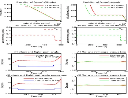
Figure 1 shows the aircraft trajectories and speeds characterized by a part of constant flight level followed by a continuous descent till the aircraft touch point. Constraints on speeds are considered, allowing a subsequent

landing on the same runway. The maximum altitudes considered are 3500 m and 4100 m for the first and

(5)

−10 −5 0

x 104 0

1000 2000 3000 4000

Evolution of Aircraft Altitudes

Lateral distance (m)

Altitude (m)

A1 altitude A2 altitude

−10 −5 0

x 104 100

150 200

Evolution of Aircraft speeds

Lateral distance (m)

Aircraft speeds (m/s)

A1 speed A2 speed

0 200 400 600

0.1 0.2 0.3 0.4 0.5 0.6

First Aircraft Throttle versus time

Time (s)

Aircraft throttle position

δx1

0 200 400 600

0.1 0.2 0.3 0.4 0.5 0.6

Second Aircraft Throttle versus time

Time (s)

Aircraft throttle position

δx2

0 200 400 600

−10 0 10 20

A1 attack and flight− path angle

Time (s)

Degrees

Attack angle Flight−path angle

0 200 400 600

−0.2 −0.1 0 0.1 0.2

A1 Roll and yaw angle versus time

Time (s)

Degrees

Roll angle Yaw angle

0 200 400 600

−10 0 10 20

A2 attack and flight− path angle versus time

Time (s)

Degrees

Attack angle Flight− path angle

0 200 400 600

−0.2 −0.1 0 0.1 0.2

A2 Roll and yaw angle versus time

Time (s)

Degrees

Roll angle Yaw angle

Figure 1. Aircraft altitudes, speeds, throttles and flight-path angles

speeds decrease from 200m/sto 69m/s. This shows the aircraft trajectory resulting from the two trajectories combination. Figure 1 shows also the two-aircraft flight-angles and throttles evolution versus time as recom-mended by ICAO during aircraft landing. As specified in this figure, the aircraft roll angles oscillate around zero. The flight-path angles are negative and bang-bang . They keep the recommended position for aircraft landing procedures. The attack angles stand between 2◦ _{and 20}◦_{. Since the trajectory of the aircraft is aligned}

with the runway, the yaw angle are small as shown in Figure 1.

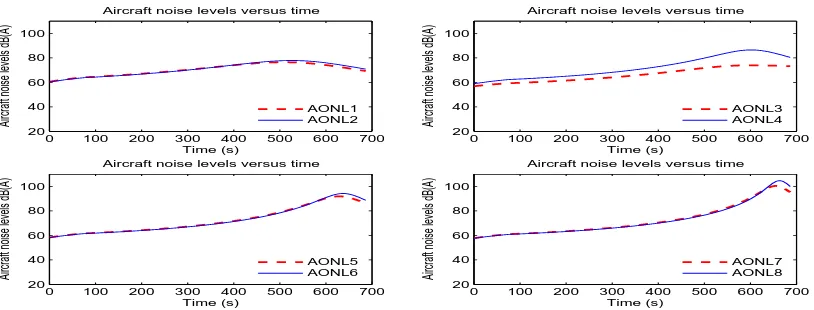
Figure 2 shows the noise levels when the optimization is applied and the solutions obtained. The obser-vation positions are (−20000 m,−20000 m,0 m) for AON L1, (−19800 m,−19800 m,0 m) for AON L2,...,

(−200m,−200m,0m) forAON L10. In this figure,AON Lmeans Aircraft Optimal Noise Level. As specified,

noise levels increase and are maximum when the observation point lies below the aircraft. Noise levels decrease gradually as the aircraft moves away from the observation point. This is in good agreement with [15, 16]. By comparison, this result is also close to standard values of jet noise on approach as shown by Harvey [2, 11, 14].

4. _Conclusion

(6)

0 100 200 300 400 500 600 700 20

40 60 80 100

Aircraft noise levels versus time

Time (s)

Aircraft noise levels dB(A)

AONL1 AONL2

0 100 200 300 400 500 600 700 20

40 60 80 100

Time (s)

AONL3 AONL4

0 100 200 300 400 500 600 700 20

40 60 80 100

Time (s)

AONL5 AONL6

0 100 200 300 400 500 600 700 20

40 60 80 100

Time (s)

AONL7 AONL8

Figure 2. Aircraft optimal noise levels

require computation of the partial derivatives of f. KNITRO is applied to perform a number of numerical experiments. An optimal local solution to the discretized problem is found through a global convergence. The obtained trajectories exhibit optimal characteristics and are effective where the noise reduction is concerned.

References

[1] L. Abdallah, Minimisation des bruits des avions commerciaux sous contraintes physiques et aérodynamique, Thèse de Mathématiques Appliquées de l’UCBL I, Septembre 2007.

[2] L. Abdallah, M. Haddou and S. Khardi, Optimization of operational aircraft parameters reducing noise emission, Applied Mathematical Sciences,4, 11(2010), 515-535.

[3] K. Blin,Stochastic conflict detection for air traffic management,Eurocontrol Experimental centre Publications Office, France, April 2000.

[4] J-L. Boiffier, The Dynamics of Flight, The Equations,SUPA ÉRO(Ecole Nationale Supérieure de l’Aéronautique et de l’Espace) et ONERA-CERT, Toulouse 25 Janvier 1999.

[5] P. Destunder, Méthodes numériques pour ingénieurs,Hermes sciences publications,12-8-2010.

[6] I. Chryssoverghi, J. Colestos and B. Kokkinis, Classical and relaxed optimization methods for optimal control problems Inter-national Mathematical Forum,2-2007N◦_{30, pp 1477-1498.}

[7] P. Faurer, Analyse num´erique, notes d’optimisation,Ellipses Marketing, 1998.

[8] A. Fortin, Analyse numérique pour ingénieurs.Troisième edition,Presses internationales polytechnique, 2008, ISBN 978-2-553-01427-7.

[9] R. Fourer, D-M. Gay and B-W. Kernigham, A modelling Language for Mathematical Programming, Second edition,Thomson Brooks[en ligne]disponible sur http://www.ampl.com,2003

[10] M-M. Harris and E. Mary, How do we Describe Aircraft Noise? NASA TM - 82712, FICAN,[en ligne] disponible sur www.fican.org.

[11] H. Harvey Hubbard, Aeroacoustics of flight vehicles, Theory and PracticesVolume 1: Noise sources and Volume 2: Noise Control. NASA Langley Research Center,Hampton, Virginia 1994.

[12] Ifrance, Fiches techniques, historiques et photos d’avions A300-600, A300-600R,[en ligne]disponible sur http://www.ifrance.com.

[13] R. James Stone, D.E. Groesbeck, C.L. Zola, An improved prediction method for noise generated by conventional profile coaxial jets,NASA TM - 82712, AIAA-81-1991 , 1991.

[14] S.Khardi F. Nahayo and M. Haddou, The Trust Region Sequential Quadratic Programming Method Applied to two-Aircraft Acoustic Optimal Control Problem,Applied Mathematical Sciences, Vol.5, No.40, pp.1953-1976, 2011, ISSN 1312-885X. [15] S. Khardi, Mathematical Model for Advanced CDA and Takeoff Procedures Minimizing Aircraft Environmental Impact,

International mathematical Forum,vol. 5, no 36, 1747 - 1774, 2010.

[16] S. Khardi, Reduction of commercial aircraft noise emission around airports. A new environmental challenge,European Confer-ence of Transport Research Institutes,vol. 1, no 4, pp 175-184, 2009.

(7)

[19] E. Roux, Pour une approche analytique de la dynamique du vol,Th`ese, SUPAERO-ONERA,Novembre 2005.

[20] E. Roux, Mod`ele de longueur de piste au d´ecollage-atterrissage, Avions de transport civil,SUPAERO-ONERA,p 345, 2006. [21] R-A. Waltz, T-D. Plantenga, Knitro Documentation Release 8.0,Ziena Optimization LLC [en ligne]disponible sur