Iranian Journal of Electrical & Electronic Engineering, Vol. 13, No. 4, December 2017 303
Utilizing Kernel Adaptive Filters for Speech Enhancement
within the ALE Framework
G. Alipoor*
(C.A.)Abstract: Performance of the linear models, widely used within the framework of adaptive line enhancement (ALE), deteriorates dramatically in the presence of non-Gaussian noises. On the other hand, adaptive implementation of nonlinear models, e.g. the Volterra filters, suffers from the severe problems of large number of parameters and slow convergence. Nonetheless, kernel methods are emerging solutions that can tackle these problems by nonlinearly mapping the original input space to the reproducing kernel Hilbert spaces. The aim of the current paper is to exploit kernel adaptive filters within the ALE structure for speech signal enhancement. Performance of these nonlinear algorithms is compared with that of their linear as well as nonlinear Volterra counterparts, in the presence of various types of noises. Simulation results show that the kernel LMS algorithm, as compared to its counterparts, leads to a higher improvement in the quality of the enhanced speech. This improvement is more significant for non-Gaussian noises.
Keywords: Speech Enhancement, Adaptive Line Enhancement, Kernel Adaptive Filtering Algorithms, Kernel Least Mean Square Algorithm, Volterra Filters.
1 Introduction1
IGNAL enhancement is one of the main problems encountered in the area of signal processing that has found various practical applications. Apart from the noise reduction, in general, this concept embraces other applications such as interference and echo cancellation. Adaptive noise cancellation (ANC) is one of the most efficient methods for speech signal enhancement. In addition to the primary noisy signal, this method requires a reference signal that is correlated to some sense to the corrupting noise and uncorrelated with the desired speech signal. In addition to simplicity and efficiency, the main advantage of this method is that it requires no prior information about the desired and noise signals. On the other hand, its main drawback is its necessity for a reference signal. However, this approach can be modified in a single-channel structure called adaptive line enhancement (ALE), in which a
Iranian Journal of Electrical & Electronic Engineering, 2017. Paper first received 31 January 2017 and accepted 13 November 2017. * The author is with the Department of Electrical Engineering, Hamedan University of Technology, Hamedan 6516913733, Iran. E-mail: [email protected].
Corresponding Author: G. Alipoor.
delayed version of the input noisy signal serves as the reference channel. This technique works by virtue of the difference between the correlation lengths of the desired and noise signals. ALE has received various applications, in particular for sonar, speech and biomedical signal processing [1].
Adaptive filters used within the ANC and ALE structures are usually based on linear algorithms such as the least mean square (LMS) and the recursive least squares (RLS) algorithms [2]. These models have satisfactory performance for Gaussian noises, but their performance deteriorates dramatically in the presence of non-Gaussian noises [3]; a phenomenon that can be seen in most practical applications. Nonlinear models, although with a higher complexity, can better extract the nonlinearities exist in the natural signals [4]. This idea has been considered somewhat, e.g. by utilizing Volterra filters [5, 6], neural networks [7, 8] and neuro-fuzzy methods [9]. In spite of their good performance in a wide range of applications, adaptive implementations of these nonlinear models suffer from the severe problems of a large number of parameters, slow convergence and the risk of being trapped in local minima. Another alternative is to use the emerging methods of kernel adaptive filters. In kernel methods, filtering is applied on the transformed data in the
S
304 Iranian Journal of Electrical & Electronic Engineering, Vol. 13, No. 4, December 2017
reproducing kernel Hilbert spaces (RKHS) that are nonlinearly related to the original input space [10, 11]. The milestone in the evolution of the kernel adaptive filtering algorithms is the kernel LMS (known as the KLMS) algorithm devised in [12].
The aim of the current study is to extend the application of the linear adaptive algorithms to nonlinear models, within the ALE structure for noise cancellation from speech signals. Among the commonly-used nonlinear models, adaptive Volterra filtering can be accomplished using kernel adaptive algorithms. In fact, it is known that Volterra series can be represented implicitly as elements of RKHSs that admit polynomial kernels [13]. In this paper kernel adaptive filters are exploited within the ALE structure for speech signal enhancement, in the presence of various types of noises, and the performance of these nonlinear algorithms are compared with that of their linear and nonlinear Volterra-based counterparts. For this purpose, the celebrated KLMS algorithm, that has attracted substantial research interests due to its simplicity and robustness, is selected. The organization of the paper is as follows. In the next section the ALE technique is described briefly. Kernel methods and the KLMS adaptive algorithm are described in section 3. Section 4 is dedicated to the simulation results. Finally some conclusion remarks are presented in section 5.
2 Adaptive Line Enhancement
In this paper noise is assumed to be additive and uncorrelated with the desired speech signal. In other words the noisy signal s kˆ
is modeled as:(1)
ˆ
s k s k n k
where s(k) and n(k) are the speech and the additive uncorrelated noise signals.
Adaptive noise cancellation, based on the structure depicted in Fig. 1, is one of the most common and efficient methods for two-channel signal enhancement that has received various applications in echo, interference and noise cancellation. The noisy speech signal s kˆ
is fed to the main channel to serve as the desired signal d(k) of the adaptive filter. The second channel receives the noise n1(k) which is correlated withn(k) and uncorrelated with s(k). The reference noise
n1(k), which is used as the input to the adaptive filter, is
adaptively filtered to make an estimate of the corrupting
w(k)
d(k)=ŝ(k)=s(k)+n(k)x(k)=n1(k)
Enhanced Signal
+
-y(k =) ñ(k)
Fig. 1 General structure for adaptive noise cancellation (ANC).
noise, denoted by n k
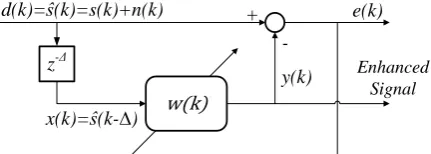
. This estimate is then subtracted from the noisy signal that acts as the desired signal of the adaptive filter, to obtain the enhanced signal. The objective is to minimize the error signal, by adaptively adjusting the filter coefficients [1].The adaptive line enhancement technique, depicted in Fig. 2, was first proposed by Widrow as an application of the ANC [1]. In the ALE a delayed version of the input signal is utilized as the secondary or reference input. This technique works by virtue of the difference between the correlation lengths of the desired and the noise signals. The principle is that the delay should decorrelate the noise, between the primary and the generated reference inputs, while leaving the speech signal correlated. In this case, it is possible for the adaptive filter to make a Δ-step-ahead prediction of s(k) based on the present and past samples of s(k-∆). However, this filter will not be able to predict n(k) from knowledge about the present and past samples of
n k . As a result, after the parameters of w(k) have converged towards their optimal values, the ALE output
y(k) is an approximated version of the desired speech signal. Successful performance of this technique depends highly on the separablity of frequency bands of the involving signals.
In general the objective of an adaptive FIR filter is to adaptively estimate the desired signal d(k)∈R based on the input vector
k x k
x k1
x k
N 1
T N
x ,
where x(k) is the input signal to the adaptive filter. At each instant this estimation can be carried out by a linear combination of the samples of this input vector, i.e. past samples of the input signal. Among the most well-known adaptive linear algorithms is the LMS algorithm [2, 14]. In practice the normalized version of this algorithm is used to alleviate the dependency of the LMS adaptive filter on the statistics of the input signal. The weight update equation for this algorithm is:
(2)
1
2
x
e k
k k k
k
w w x
0 < μ ≪ 1 is the convergence parameter to control the memory span of the predictor filter and therefore the convergence speed of the algorithm and 2
x k
is an estimate of the input signal variance that can be updated sequentially as:w(k)
d(k)=ŝ(k)=s(k)+n(k)
y(k)
e(k) +
-z-Δ Enhanced
Signal
x(k)=ŝ(k-∆)
Fig. 2 General structure for adaptive line enhancement (ALE).
Iranian Journal of Electrical & Electronic Engineering, Vol. 13, No. 4, December 2017 305
(3)
22 2
1 1 1
x k x k x k
β is a forgetting factor affecting the memory of this estimation.
3 Kernel LMS 3.1 Kernel Methods
It can be shown that for any RKHS H with the kernel function K, one can imagine a space, known as the feature space, in which the inner product can be calculated through evaluating its kernel function in the original input space [10, 11]. In other words, representing the function
x K
x, as
xi , the kernel K corresponds to a feature mapping
for which:(4)
k, l
k , l , k, lK x x
x
x x x In kernel adaptive filtering, at each instant k, the input vector x(k) is assumed to be mapped into the transformed data φ(x(k)). Then, if for simplicity we denote φ(x(k)) by φ(k), the desired signal d(k) is estimated by linear combination of the samples of the transformed data φ(k). Calculation in the high-dimensional feature space can be done by reformulating the original linear algorithms in terms of the inner products and then replacing the inner products with the kernel function evaluations in the original space. This will be equivalent to implicitly solving the linear adaptive algorithms in the feature spaces induced by the kernel functions, where transformed input signals are more likely to be linearly related to the so-called desired signal. The resultant algorithms possess the properties of convexity and universal nonlinear approximation. Furthermore, nonlinear kernel methods are quite flexible so that one can change the nonlinear model just by changing the kernel function used.
3.2 Extending the LMS Algorithm into the RKHS
The normalized KLMS algorithm [12, 15] can be derived by employing the normalized LMS algorithm to predict the desired signal {d(1), d(2), ⋯} based on the transformed input vector {φ(1), φ(2), ⋯} as:
(5)
2
1
1
T
e k d k k k
e k
k k k
k ω φ
ω ω φ
where ω(k) is the filtering coefficients vector in the feature space at instant k. Since φ φk, k K
x xk, k
, one can sequentially update
2
k , i.e. the estimate ofthe input signal variance in the feature space, as:
2 2
1 1 k, k
k k K
x xAssuming ω(0) = 0, it is easy to see that:
(6)
2
1 k l e l k l l
ω φAt instant k, having the coefficients vector ω(k-1), the filter’s output can be written as:
(7)
1 2 1 1 k T T l e ly k k k l k
l
ω φ φ φ
which is efficiently computed using the kernel trick in the input space as:
(8)
1
2
1
, k
l k
l
e l K y k l
x xIn other words, it is possible to compute the output of the filter without direct access to its coefficients in the high-dimensional feature space. However, it is necessary to retain the input vectors x(l) along with the corresponding coefficients e
l /
2
l in a set calleddictionary. The resultant algorithm, called normalized kernel LMS, or shortly KLMS, is summarized in Table 1. It has been shown that the KLMS algorithm possesses the property of self-regularization that makes an extra regularization unnecessary [15]. In addition to simplifying the implementation, this property improves the performance, because regularization biases the optimal solution.
3.3 Sparsification
Essentially the size of the network over which the signal is expanded, or the number of past samples based on which the signal is estimated, increases with the size of the data, as a result of the representer theorem [16]. This phenomenon is also clear from the KLMS algorithm, where the size of the dictionaries x
kand e
k grow linearly with the time. In practice, redundancy among input data makes it possible to drastically reduce the size of the memory, at the cost ofTable 1 The normalized KLMS algorithm.
2 2 1 2 1 2 2 2 11 1 , 1 1 , 1 1 / 1 2, 3,
,
1 1 ,
1 , 1 , /
x e
k
l
x x
e e
a small positive number
e x e
k
e l
e k d k K l k
l
k k K k k
k k k
k k e k
fo k end r
x x x x x x306 Iranian Journal of Electrical & Electronic Engineering, Vol. 13, No. 4, December 2017
a negligible effect on the quality of the model. This is generally carried out based on selecting, based on a measure, the most informative data and discarding the others from the dictionary. This procedure is termed sparsification and many techniques have been proposed for this purpose. One of the first and still widely used measures is the novelty criterion (NC) proposed in [17] which acts based on a simple distance measure in the input space. In NC, at iteration k, the minimum distance of the new input vector x(k) to all the vectors retained in the dictionary x
k1
(i.e. x 1
min
l k k l
x x x ) is
first calculated. The new input vector will be accepted as a new element of the dictionary only if this measure is larger than a preset threshold (say δ1), and the
estimation error e(k) is also larger than another preset threshold (say δ2).
4 Results
To alleviate the drawbacks of the commonly-used adaptive nonlinear models, the kernel adaptive filters are utilized within the ALE structure for speech signal enhancement. Due to its appealing properties, the normalized kernel LMS algorithm is adopted for this purpose. To show its usefulness, this algorithm is compared with its linear as well as nonlinear Volterra counterparts. The KLMS algorithm is utilized with a quadratic kernel, including the first-order term. Defining the first and second-order input vectors as
(9)
1
2
1 1
2 2
1 1
1 1
T N
T N
k x k x k x k N
k x k x k x k N
x
x
respectively, this quadratic kernel can be described as
(10)
1 2 1 2
2
1 1 2 2
, , ,
T T
K l l k k
l k l k
x x x x
x x x x
N1 and N2 are the memory spans of the first and
second-order terms. This kernel is defined in a general form to make it possible to distinguish between memory spans of the linear and quadratic terms.
In these testes, N1 as well as N, i.e. the memory span
of the linear LMS algorithm, are set to 10, but N2 is set
to 5. Volterra LMS (VLMS) algorithm is also considered using a quadratic kernel identical to that of the KLMS algorithm with the same parameters, i.e.
N1=10 and N2=5. The best values for other parameters,
for each algorithm, are chosen based on an exhaustive search over some ranges of possible choices. To this end, in all experiments, the convergence parameter μ and the forgetting factor β are set to 0.0005 and 0.9, respectively. For the KLMS algorithm, novelty criterion is used for sparsification, with the distance threshold
δ1=0.2 and the error threshold δ2=0.1. Using NC, less
than 10% of the input vectors are retained in the dictionary, on average, at the end of processing a speech signal. All the results reported throughout this paper are averaged over all 504 SI speech signals in the test set of the DARPA TIMIT corpus [18]. These signals have an average length of about 3.5 seconds containing each a whole sentence in English, uttered by both male and female speakers. They were originally sampled at 16 kHz and are down-sampled to 8 kHz, after applying a 20th order anti-aliasing low-pass filter, and then quantized uniformly at 16 bps.
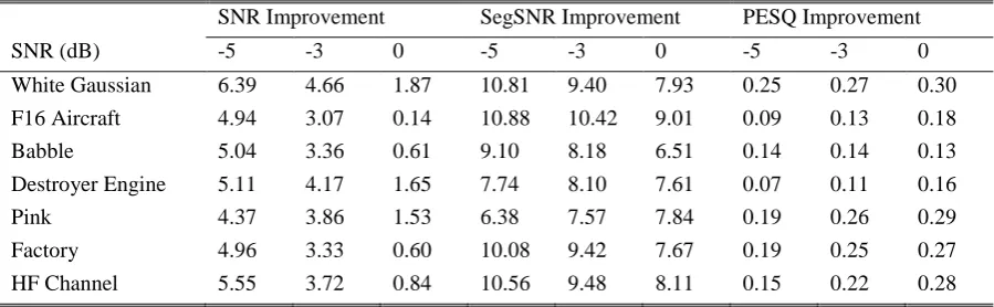
Various noise signals were first added to the speech signals at several signal-to-noise-ratio (SNR) levels and the ALE is then used to enhance the noisy signals. These noise signals are the white Gaussian, pink and high frequency channel noises as well as natural sounds of the factory, F16 aircraft, destroyer engine and babble. The comparison is drawn based on improvement in three criteria of SNR, segmental SNR (SegSNR) and PESQ. Segmental SNR is calculated by averaging the short-time SNRs computed on segments of 20 ms (160 samples) length. PESQ measure is evaluated as suggested by the ITU-T P.862 recommendation [19] that has a good correlation with the subjective measure of mean opinion score (mos).
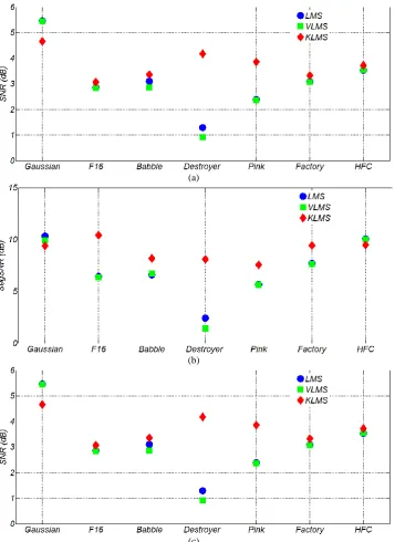
Average results for improvement in the quality of the noisy speech signals, using the LMS, VLMS and KLMS adaptive algorithms, are summarized in Tables 2-4. These tests have been launched in the presence of various noises with three SNR levels of 0, -3 and -5 dB. As one can see from these results, higher improvement can be achieved using nonlinear kernel-based LMS algorithm. This improvement is more considerable with non-Gaussian noises. This is while the nonlinear Volterra-based model does not result in a considerable improvement, as compared to the linear algorithm. This is mainly due to the shortcomings the adaptive Volterra filters suffer from, in particular the slow convergence. The better performance of the kernel-based model can be more clearly observed from Fig. 3 in which the average improvement achieved by the KLMS algorithm is compared against that of the LMS and the VLMS algorithms, at the noise level of -3 dB. Some marker symbols are hidden, in this figure, below the other symbols.
These results are in agreement with the argument provided on the linear and nonlinear adaptive filtering algorithms. In fact, although linear models have satisfactory performance for Gaussian noises, their performance deteriorates dramatically in the presence of non-Gaussian noises [3]. Therefore it is reasonable to expect nonlinear adaptive filters to result in a better performance, in presence of non-Gaussian noises. In other words, nonlinear models, although with a higher complexity, can better extract the nonlinearities exist in the natural signals [4]. In spite of their good performance in a wide range of applications, adaptive implementations of nonlinear Volterra filters suffer
Iranian Journal of Electrical & Electronic Engineering, Vol. 13, No. 4, December 2017 307
Table 2 Average improvements obtained by means of the LMS algorithm for various noises at three SNR levels.
SNR Improvement SegSNR Improvement PESQ Improvement SNR (dB) -5 -3 0 -5 -3 0 -5 -3 0 White Gaussian 6.99 5.46 3.12 11.53 10.32 8.46 0.15 0.18 0.22 F16 Aircraft 4.43 2.86 0.26 7.24 6.42 5.01 0.00 -0.02 -0.05 Babble 4.56 3.10 0.69 7.48 6.61 5.14 -0.09 -0.07 -0.04 Destroyer Engine 1.99 1.29 -0.13 2.80 2.42 1.69 -0.01 -0.02 -0.04 Pink 3.76 2.39 0.01 6.46 5.66 4.30 0.01 0.03 0.04 Factory 4.78 3.09 0.38 8.70 7.69 6.03 0.02 0.03 0.03 HF Channel 5.39 3.53 0.68 11.30 10.07 8.11 -0.09 -0.08 -0.04
Table 3 Average improvements obtained by means of the VLMS algorithm for various noises at three SNR levels.
SNR Improvement SegSNR Improvement PESQ Improvement SNR (dB) -5 -3 0 -5 -3 0 -5 -3 0 White Gaussian 6.88 5.44 3.15 10.84 9.89 8.30 0.16 0.19 0.23 F16 Aircraft 4.37 2.83 0.25 7.15 6.37 4.99 0.00 -0.02 -0.06 Babble 4.44 2.87 0.27 7.60 6.71 5.18 -0.07 -0.08 -0.08 Destroyer Engine 1.23 0.91 0.18 1.66 1.44 0.99 0.05 0.05 0.04 Pink 3.72 2.37 0.01 6.41 5.64 4.29 0.01 0.03 0.03 Factory 4.74 3.07 0.38 8.60 7.63 6.00 0.01 0.02 0.02 HF Channel 5.39 3.54 0.69 11.24 10.04 8.10 -0.09 -0.08 -0.04
Table 4 Average improvements obtained by means of the KLMS algorithm for various noises at three SNR levels
SNR Improvement SegSNR Improvement PESQ Improvement SNR (dB) -5 -3 0 -5 -3 0 -5 -3 0 White Gaussian 6.39 4.66 1.87 10.81 9.40 7.93 0.25 0.27 0.30 F16 Aircraft 4.94 3.07 0.14 10.88 10.42 9.01 0.09 0.13 0.18 Babble 5.04 3.36 0.61 9.10 8.18 6.51 0.14 0.14 0.13 Destroyer Engine 5.11 4.17 1.65 7.74 8.10 7.61 0.07 0.11 0.16 Pink 4.37 3.86 1.53 6.38 7.57 7.84 0.19 0.26 0.29 Factory 4.96 3.33 0.60 10.08 9.42 7.67 0.19 0.25 0.27 HF Channel 5.55 3.72 0.84 10.56 9.48 8.11 0.15 0.22 0.28
from severe problems of a large number of parameters, slow convergence and the risk of being trapped in local minima. Nonetheless, kernel methods are emerging solutions that can tackle these problems by extending linear algorithms to reproducing kernel Hilbert spaces created by nonlinear mapping of the original input space. This in turn results in a better performance of the kernel adaptive algorithms, in particular in the presence on non-Gaussian noises.
5 Conclusions
Adaptive filters used within the ALE structure are usually based on linear algorithms that have not satisfactory performance in the presence of non-Gaussian noises. The aim of the current study was to extend the application of the linear adaptive algorithms
to nonlinear models, within the ALE structure for noise cancellation from speech signals. One of the commonly-used solutions is to utilize the Volterra filters. However, adaptive implementations of these models suffer from severe problems of large number of parameters and slow convergence. On the other hand, adaptive Volterra filtering can be accomplished using kernel adaptive algorithms.
The main contribution of this paper was to alleviate drawbacks of the nonlinear models within the ALE structure for speech signal enhancement, by way of utilizing the kernel adaptive filters. For this purpose, the celebrated KLMS algorithm, that has attracted substantial research interests due to its simplicity and robustness, was selected. Performance of this kernel adaptive algorithm was compared to that of their linear
308 Iranian Journal of Electrical & Electronic Engineering, Vol. 13, No. 4, December 2017 (a)
(b)
(c)
Fig. 3 3Average improvements obtained by means of the KLMS, LMS and VLMS algorithms, at the noise level of -3 dB, for a) SNR, b) Segmental SNR and c) PESQ measures.
and nonlinear Volterra-based counterparts, i.e. the LMS and VLMS algorithms. Simulation results revealed that, higher improvement can be achieved using nonlinear kernel-based LMS algorithm. This improvement in performance was considerably higher for non-Gaussian noises. This is while the nonlinear Volterra-based model does not result in a considerable improvement, as compared to the linear algorithm.
The current study showed the capability of the KLMS algorithm in dealing with non-Gaussian interfering signals. Evaluating other nonlinear kernel adaptive filtering algorithms within the ALE structure as well as
utilizing these algorithms in the more general framework of the ANC for noise, interference and echo cancellation remain some topics for future studies.
Acknowledgment
The author would like to thank Hamedan University of Technology (HUT) for funding this research under Contract No. 16/92/3/P/517.
Iranian Journal of Electrical & Electronic Engineering, Vol. 13, No. 4, December 2017 309 References
[1] B. Widrow, et al., “Adaptive noise cancelling: Principles and applications,” Proceedings of the IEEE, Vol. 63, pp. 1692-1716, 1975.
[2] S. Haykin, Adaptive Filter Theory, Pearson Education India, 2008.
[3] A. Hussain, et al., “Nonlinear Speech Enhancement: An Overview,” in Progress in
Nonlinear Speech Processing, Springer Berlin
Heidelberg, 2007, pp. 217-248.
[4] M. Faundez-Zanuy, et al., “Nonlinear speech processing: overview and applications,” Control and
intelligent systems, Vol. 30, pp. 1-10, 2002.
[5] V. H. Diaz-Ramirez and V. Kober, “Robust speech processing using local adaptive non-linear filtering,”
IET Signal Processing, Vol. 7, pp. 345-359, 2013.
[6] Z. Zhao, et al., “A New Variable Step Size NLMS Algorithm Based on Decorrelation for Second-Order Volterra Filter,” Advances in Automation and
Robotics, Vol. 1, p. Springer, 2011.
[7] W. G. Knecht, et al., “Neural network filters for speech enhancement,” IEEE Transactions on Speech
and Audio Processing, Vol. 3, pp. 433-438, 1995.
[8] S. A. Vorobyov and A. Cichocki, “Hyper Radial Basis Function Neural Networks for Interference Cancellation with Nonlinear Processing of Reference Signal,” Digital Signal Processing, Vol. 11, pp. 204-221, 2001.
[9] J. Chia-Feng and L. Chgin-Teng, “Noisy speech processing by recurrently adaptive fuzzy filters,”
IEEE Transactions on Fuzzy Systems, Vol. 9, pp.
139-152, 2001.
[10]J. Shawe-Taylor and N. Cristianini, Kernel Methods
for Pattern Analysis. Cambridge, UK: Cambridge
University Press, 2004.
[11]B. Schölkopf and A. Smola, Learning with Kernels:
Support Vector Machines, Regularization,
Optimization and Beyond Cambridge, MA: MIT
Press, 2002.
[12]P. Pokharel, et al., “Kernel LMS,” in International Conforence of Acoustics, Speech, Signal Process.
(ICASSP), Vol. 3, pp. III-1421–III-1424, 2007.
[13]M. O. Franz and B. Schölkopf, “A Unifying View of Wiener and Volterra Theory and Polynomial Kernel Regression,” Neural Computation, Vol. 18, pp. 3097-3118, 2006.
[14]M. Tummala and B. V. Rao, “A study of LMS and SER algorithms for FIR filtering,” Computers &
Electrical Engineering, Vol. 13, pp. 169-175, 1987.
[15]W. Liu, et al., “The Kernel Least Mean Square Algorithm,” IEEE Transactions on Signal
Processing, Vol. 56, pp. 543–554, 2008.
[16]J. Mercer, “Functions of positive and negative type and their connection with the theory of integral equations,” Philosophical Transactions of the Royal
Society, pp. 415-446, 1909.
[17]J. Platt, “A Resource Allocating Network for Function Interpolation,” Neural Computation, Vol. 3, pp. 213–225, 1991.
[18]J. S. Garofolo, et al. DARPA TIMIT Acoustic Phonetic Continuous Speech Corpus CDROM
[Online].
[19]ITU-T, “P.862: Perceptual evaluation of speech quality (PESQ): An objective method for end-to-end speech quality assessment of narrow-band telephone networks and speech codecs,” in ITU-T
Recommendation, ed. Geneva, Switzerland, 2001.
G. Alipoor received his BSc in telecommunication engineering in September 2002 from Tabriz University and his MSc and PhD in electronic engineering in September 2005 and September 2012, respectively, both from Shahid Beheshti University. He was with Kermanshah Petrochemical Industrial Company (KPIC) as a senior instrument engineer from October 2005 for two years. He has been an assistant professor at the Hamedan University of Technology, from September 2012. His main research interests include nonlinear adaptive filters as well as the utilizing of modern signal representation approaches in speech and audio signal processing, especially for analysis and recognition.