Linear and Nonlinear Multivariate Classification of
Iranian Bottled Mineral Waters According to Their
Elemental Content Determined by ICP-OES
J.B. Ghasemi,
1,*E. Zolfonoun,
1and R. Khosrokhavar
21Department of Chemistry, Faculty of Sciences, K.N. Toosi University of
Technology, Tehran, Islamic Republic of Iran
2Food and Drug Laboratory Research Center, MOH & ME, Tehran, Islamic Republic of Iran
Received: 1 February 2012 / Revised: 22 December 2012 / Accepted: 2 February 2013
Abstract
The combinations of inductively coupled plasma-optical emission spectrometry
(ICP-OES) and three classification algorithms, i.e., partial least squares
discriminant analysis (PLS-DA), least squares support vector machine (LS-SVM)
and soft independent modeling of class analogies (SIMCA), for discriminating
different brands of Iranian bottled mineral waters, were explored. ICP-OES was
used for the determination of Li, Na, K, Ca, Mg, Sr, Ba, B, Si and Zn in bottled
mineral waters (150 samples) from 30 brands. Hierarchical cluster analysis (HCA)
and principal component analysis (PCA) showed differences in water samples
according to the mineral composition. 120 samples (4 for each brand) were
selected randomly for the calibration set, and 30 samples (1 for each brand) for the
prediction set. PLS-DA, LS-SVM and SIMCA were implemented for calibration
models. The results suggest that ICP-OES combined with PLS-DA, LS-SVM and
SIMCA models had the capability to discriminate the different brands of mineral
waters with high accuracy. The model can resolve the tap water samples from
classified mineral waters accordingly.
Keywords: Multivariate classification; Inductively coupled plasma optical emission
spectrometry; Bottled mineral waters
* Corresponding author, Tel.: +98(21)22850266, Fax: +98(21)22853650, E-mail: [email protected] Introduction
Drinking water, as the most important type of natural water, has a dominating role in human life. It is one of the basic and most inspected nourishment components therefore great demands are imposed on its quality. The world market of bottled water has grown quickly and is considered as a global billion dollar business [1-3]. In
waters have beneficial medicinal and therapeutic effects [5]. Almost any mineral species are allowed to be contained in drinking water. It is demanded that they are not harmful to the human body and in addition, they should be biologically valuable. Drinking water originating from a natural source has to fulfil specified health and technical requirements [6, 7]. It should be tasty, with a good appearance, adequate temperature, refreshing and without any odour. With regard to its biological and bacteriological properties it must not contain any disease-carrying germs. Drinking water should contain many species, mainly trace biogenic elements, in such an amount and composition that their optimal utility for human body is assured. Trace elements can be categorized as those essential to human life, e. g. Co, Cr, Cu, Fe, Mn, Mo, Se, and Zn, and those potentially toxic, e.g. Ag, Al, As, Cd, Pb, and Ni. The presence of non-essential and toxic elements does not necessarily indicate that water consumption presents a health risk. Also, certain essential trace elements, like Co, Cr, Fe, Mn, and Se, can be toxic at concentrations above the specific cutoff levels [8]. Therefore it is necessary to follow the presence and concentration of species important for a proper advancement and growth of the human body. Application of multivariate analysis to complex data sets are enjoying in the last years a high scientific interest and are now routinely used in most fields of application [9-11]. One of the main advantages of these techniques, such as principal component analysis (PCA), factor analysis (FA), cluster analysis (CA), is in the ability in analyzing large and complicated data, which have many variables and experimental units. Such methods sometimes create new variables by reducing the number of original variables in the comparison and interpretation of the data [12]. PCA, FA, and CA will find groups and sets of variables with similar properties, thus might allow us to simplify our description of observations by finding the structure or patterns in the presence of chaotic or confusing data. These techniques besides allow to elaborate data from not homogeneous variables, giving so the possibility to contemporarily consider chemical, physicals and microbiological parameters. This ability allows to evaluate the potential correlations among the parameters and to exploit these correlations for analytical purposes [13-16]. Multivariate methods have been often used for the classification and comparison of different samples of waters [17-19]. Güler [2] classified 130 Turkish bottled water brands by using multivariate pattern recognition methods. The production licenses provided information on up to 34 physico-chemical parameters were used as database. The relationships among eight selected major ion chemistry variables (calcium,
magnesium, sodium, potassium, chloride, sulfate, bicarbonate, and fluoride) were examined by principal components analysis and hierarchical cluster analysis. Yekdeli-Kermanshahi and co-workers [17] investigated the chemical composition of Iranian bottled water brands by correlation analysis, principal component analysis and hierarchical cluster analysis. For this purpose, the chemical composition reported on the label of 73 Iranian bottled waters was used as data set. It was found out that only 26 brands had eight important parameters such as calcium, magnesium, potassium, sodium, chloride, sulphate, bicarbonate and fluoride and 20 brands had acceptable charge balance error. Results showed that Iranian bottled waters can be divided into 11 classes. Lourenço and co-workers [18] used from principal component analysis to identify the main geotectonic interrelationships among physicochemical parameters, enhancing similarities and dissimilarities, and contributing to a new typology of 33 different types of Portugalian bottled waters, based on their hydrochemical characteristics and geological occurrence. Kraic and co-workers [19] categorized ninety-three water samples originated from four European countries into five classes as the tap, mineral, mineral carbonated, spring, and spring carbonated water. Analytical measurements were performed by inductively coupled plasma-mass spectrometry. Different water categories were characterized by chemometrical techniques, mainly by principal compo-nent analysis, cluster analysis, linear and quadratic discriminant analyses, correlation analysis, and ANOVA. The classification results were successful and close to 100 %, which was proved by the leave-one-out cross-validation procedure. Versari and co-workers [3] characterized bottled mineral waters (132 samples) from 19 districts of Italy by means of the physico-chemical and chemical composition (30 parameters) reported on their label by using statistical analysis. The relationships among 12 selected variables were examined by princi-pal component analysis; then, hierarchical cluster analy-sis was used to search the ‘‘natural’’ grouping among the mineral waters, and linear discriminant analysis allowed to check the reliability of classification.
Materials and Methods
Reagents and Samples
All reagents used were of analytical reagent grade (Merck, Germany). Double-distilled deionized water was used through all the experiments. Stock standard solutions of Li, Na, K, Ca, Mg, Sr, Ba, B, Si and Zn (1000 µg mL−1) were purchased from Sigma-Aldrich Company (USA). This solution was appropriately diluted in double-distilled deionized water for prepared metals standard calibration solutions. Different brands of mineral water samples were obtained from local stores, representing the common types readily available to consumers. Three tap water samples were collected from different area of the Tehran city.
Instrumentation and Software
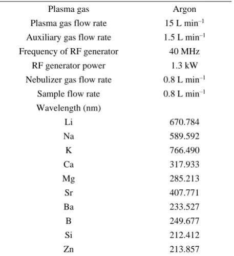
Elemental analysis was carried out using a Varian (Vista-MPX) simultaneous ICP-OES coupled to a concentric nebulizer and equipped with a charge coupled device (CCD) for determination of the metal ions. Operational conditions and selected wavelengths for the metal ions were optimized and summarized in Table 1. Initially 39 elements (Ag, Al, As, Au, B, Ba, Be, Bi, Ca, Cd, Ce, Co, Cr, Cu, Fe, Ga, Hg, In, K, La, Li, Mg, Mn, Mo, Na, P, Pb, Pd, Rh, Sb, Sc, Se, Si, Sn, Sr, Te, Tl, V and Zn) were analyzed but some of them were below the quantification limits, and therefore the methodology was reduced to 10 elements (Li, Na, K, Ca, Mg, Sr, Ba, B, Si and Zn). In Table 2, the ICP-OES results for one sample from each brand are presented. The data were processed on a Toshiba computer with Pentium ΙV as central processing unit (2 Gb RAM) using MATLAB software, version 7.7. PCA, HCA, DA and SIMCA were carried out using PToolbox, version 5.2 (Eigenvectors Company). The LS-SVM optimization and model results were obtained using the LS-SVM lab toolbox version 1.5 (Matlab toolbox for least-squares support vector machines).
Multivariate Classification
Non-Supervised Methods
Non-supervised methods, also known as exploratory methods, do not require any a priori knowledge about the group structure in the data, but instead produce the grouping, i.e. clustering, themselves. This type of analysis is often very useful at an early stage of the investigation to explore subpopulations in a data set. Cluster analysis can be performed with simple visual
techniques, such as hierarchical cluster analysis or principal component analysis.
Principal Component Analysis (PCA)
PCA is a well-known statistical method for reducing the dimensionality of data sets [11]. PCA is the simplest of the true eigenvector-based multivariate analyses. Often, its operation can be thought of as revealing the internal structure of the data in a way which best explains the variance in the data. If a multivariate data set is visualized as a set of coordinates in a high-dimensional data space (1 axis per variable), PCA supplies the user with a lower-dimensional picture, a “shadow” of this object when viewed from it is (in some sense) most informative viewpoint. PCA involves the calculation of the eigenvalue decomposition of a data covariance matrix or singular value decomposition of a data matrix, usually after mean centering the data for each attribute. The results of a PCA are usually discussed in terms of component scores and loadings. This approach has been used to extract related variables and infer the processes that control water chemistry [2,3].
Hierarchical Clustering Analysis (HCA)
Hierarchical cluster analysis (HCA)’s primary goal is to display the data in such a way as to emphasize their natural clusters and patterns in a two dimensional space.
Table 1. Operating parameters for ICP-OES
Plasma gas Argon
Plasma gas flow rate 15 L min–1
Auxiliary gas flow rate 1.5 L min–1
Frequency of RF generator 40 MHz RF generator power 1.3 kW
Nebulizer gas flow rate 0.8 L min–1
Sample flow rate 0.8 L min–1
Wavelength (nm)
Li 670.784
Na 589.592
K 766.490
Ca 317.933
Mg 285.213
Sr 407.771
Ba 233.527
B 249.677
Si 212.412
The results, qualitative in nature, are usually presented in the form of a dendrogram, allowing the visualization of clusters and correlations among samples or variables [20, 21]. In HCA, the Euclidean distance is selected as the similarity measurement, which is straight line distance between two points in c-dimensional space defined by c number of variables.
Supervised Methods
In the supervised methods each sample is formerly assigned to a definite class. For building a supervised classification model,a set of sample objects with known classes is needed. This set of known objects is called the training set because it is used by the classification programs to learn how to classify objects. There are two phases to construct a classifier. In the training phase, the training set is used to decide how the parameters ought to be weighted and combined in order to separate the various classes of objects. In the prediction phase, the weights determined in the training set are applied to a set of objects that do not have known classes in order to determine what their classes are likely to be. Partial least squares discriminant analysis (PLS-DA), least squares support vector machine (LS-SVM) and soft independent modeling of class analogies (SIMCA) are of most commonly used supervised classification methods.
Soft Independent Modeling of Class Analogies (SIMCA)
Soft independent modeling of class analogies (SIMCA) is a well known and widely used supervised classification technique introduced by Wold [22, 23]. Its main idea is to build a PCA model for each class belonging to a training set. Each borderline of these models is determined by multiplying the average reference sample deviation from the model with the appropriate F value (corresponding degrees of freedom and selected level of significance). Subsequently, new samples (test samples) can be fitted to these models. By comparing the residuals to the maximum allowed residuals (the borderline of the model), test samples can be classified. In this study, optimum component of PC model is determined for each class by the validation set.
Partial Least Squares Discriminant Analysis (PLS-DA)
This classification method is based on a PLS regression where class membership is the property [24-26]. Linear discriminant analysis would traditionally have been the most appropriate technique to classify the data, given that the data were normally distributed [24].
However formal linear discriminant analysis usually cannot be performed due to the large number of variables in the training dataset relative to the amount of measurements taken. A reduction in data dimensionality therefore is needed to avoid overfitting before continuing with the classification. PLS-DA therefore is preferred to analyze the data. The first step in this technique is a dimension reduction by using partial least
Table 2. ICP-OES results for one sample from each brand
Class Concentration (µg mL
–1)
Li Na K Ca Mg Sr Ba B Si Zn
1 0.008 1.407 0.392 26.18 6.165 0.101 0.003 0.031 2.667 0.000
2 0.010 6.619 0.554 61.85 12.25 0.309 0.163 0.064 6.829 0.000
3 0.004 3.469 0.140 21.59 2.754 0.090 0.002 0.035 8.142 0.055
4 0.021 10.39 0.871 49.02 16.84 0.689 0.023 0.051 6.145 0.000
5 0.006 2.219 0.705 35.84 14.89 0.683 0.039 0.028 2.854 0.000
6 0.008 48.26 0.075 14.56 6.682 0.272 0.004 0.273 3.962 0.000
7 0.011 11.75 1.978 15.85 3.150 0.086 0.030 0.041 33.67 0.160
8 0.005 7.785 0.467 58.83 8.342 0.518 0.064 0.023 7.801 0.024
9 0.002 12.35 0.709 0.287 11.13 0.001 0.003 0.090 0.170 0.000
10 0.007 3.926 1.093 7.322 1.690 0.056 0.002 0.026 15.85 0.010
11 0.002 0.961 0.256 33.46 5.995 0.083 0.005 0.025 2.202 0.000
12 0.005 3.137 0.546 57.05 4.225 0.208 0.019 0.026 6.286 0.000
13 0.000 6.408 0.572 81.72 7.521 0.336 0.008 0.068 11.17 0.029
14 0.004 46.89 0.081 18.04 5.896 0.239 0.007 0.295 3.618 0.000
15 0.022 25.86 0.638 27.02 20.4 0.245 0.004 0.090 6.404 0.011
16 0.003 23.37 3.372 39.74 6.230 0.218 0.064 0.141 23.53 0.071
17 0.008 24.84 0.459 30.47 5.634 0.253 0.014 0.075 3.638 0.054
18 0.002 14.68 0.486 45.12 5.954 0.128 0.016 0.027 2.729 0.000
19 0.004 26.33 0.831 26.56 6.987 0.230 0.009 0.074 1.247 0.000
20 0.001 0.259 0.169 45.18 3.154 0.117 0.006 0.019 2.502 0.000
21 0.000 0.239 0.301 55.67 1.969 0.108 0.009 0.013 2.881 0.000
22 0.003 3.226 0.624 39.69 5.629 0.137 0.012 0.032 3.952 0.038
23 0.028 34.51 2.098 42.20 11.76 0.520 0.149 0.124 5.082 0.000
24 0.005 3.524 0.992 55.06 11.63 0.203 0.033 0.021 6.490 0.000
25 0.001 0.369 0.238 33.44 7.691 0.079 0.031 0.000 2.126 0.000
26 0.006 25.07 1.015 15.97 6.564 0.211 0.004 0.971 3.511 0.000
27 0.014 29.03 2.912 11.13 21.75 0.357 0.021 0.434 5.283 0.000
28 0.012 82.40 2.614 50.14 21.84 0.658 0.020 0.293 7.855 0.156
29 0.007 11.09 0.387 51.07 13.09 0.723 0.058 0.099 8.059 0.054
30 0.004 11.38 0.837 49.70 5.662 0.362 0.035 0.016 3.570 0.018
31 0.004 17.91 0.581 60.88 10.12 0.370 0.034 0.049 8.806 0.049
32 0.007 10.53 0.564 42.15 5.823 0.388 0.032 0.048 3.109 0.116
squares (PLS). PLS is comparable to the commonly used dimension reduction technique of principal component analysis (PCA), with the important difference being that PLS explains both sample variation and response variation. In contrast with PCA, PLS components are chosen such that the sample covariance between the response and a linear combination of the predictors is maximized. A component with a small predictor variance could be a better predictor of the response classes, a fact which is not taken into account in PCA. The main objective of partial least squares is to build a model which relates the response variables to the factor scores multiplied by their loadings. The factor scores, in turn, are linear combinations of the original predictor variables, resulting in no correlation between the factor score variables used in the predictive regression model:
Y=TQ+E
where Y = n × m response variables matrix
T = factor score matrix (=predictor variables x weights)
Q = coefficients matrix (=loadings for T)
E = n × m noise term
The second step in the PLS-DA technique involves a classification using linear discriminant analysis (LDA). LDA is well-known as a classification technique based on the gross variability ‘within groups’ and ‘among groups’. The combination of PLS and LDA therefore results in a dimension reduction as well as a classification outcome. A cross-validation method was chosen in order to evaluate the model obtained by PLS-DA. The basic precept behind this model validation technique is that a data subset (test data) is removed before training begins. The performance of the selected model then can be tested on the new test data. The number of latent variables where then specified that had to be retained in the model, which relates to the percent variance captured by the model in X and Y.
Support Vector Machines (SVM)
The SVM [27,28] is a supervised method that has been applied to a large range of pattern recognition problems. The aim of SVM is to find an optimal hyperplane (classifier) that correctly separates objects of the different classes as much as possible. This is done by leaving the largest possible fraction of points of the same class on the same side and maximizing the distance of either class from the hyperplane. It is based on structural risk minimum mistake instead of the minimum mistake of the misclassification on the
training set that SVM can effectively avoid over-fitting problem. Due to its advantages and remarkable generalization performance over other methods, SVM has attracted attention and gained extensive applications [28]. As a simplification of traditional of SVM, Suykens and Vandewalle [29] have proposed the use of least-squares SVM (LS-SVM). LS-SVM encompasses similar advantages as SVM, but its additional advantage is that it requires solving a set of only linear equations (linear programming), which is much easier and computationally more simple. The theory of LS-SVM has also been described clearly by Suykens et al. [29, 30] and application of LS-SVM in quantification and classification reported by some of the workers [32, 33]. The standard SVM are designed for binary classification. How to effectively extend it for multi-class multi-classification is still on-going issue. Currently, there are two types of approaches for multi-class SVM classification. One is by constructing and combining several binary classifiers such as against-all, one-against-one, and complete-code while the other is by directly considering all data in one single optimization formulation.
Model Efficiency Estimation
For the evaluation of the performance of multivariate classification models, the correct classification rate (CCR) was used [34]:
1Correctly classified samples in class i
Total number of samples in class i
CCR=kj 100
where k is the total number of classes.
Results and Discussion
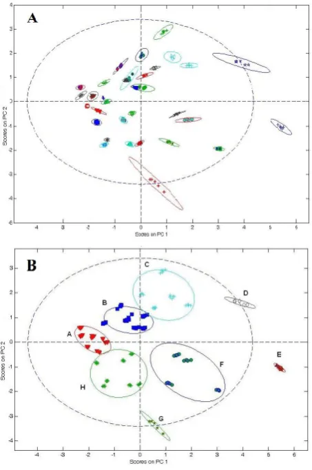
Principal Component Analysis
different classes according to their mineral content (Fig. 2 (B)). The 26 mineral water brands with normal-mineral content were grouped on the left side and center of the plot. As Fig. 2 shows, three mineral water brands (23, 28 and 26) are clearly different from the others (classes D, E and G). Classes 23 and 28 have high concentration of Na, Ca and Mg whereas class 26 has high concentration of B. Also this figure shows that tap water samples (31, 32 and 33) and four mineral water brands are localized in a special class (class B) and are different from the other mineral water brands.
Hierarchical Clustering Analysis
Hierarchical cluster analysis (HCA) was used for searching the natural grouping among bottled waters from different brands. The bottled water brands were classified according to their major ion composition. The data were standardized (z-scores) and the Euclidean distance was used as similarity measurement. The Ward’s method was used to obtain hierarchical associations. The result of the HCA is presented as a dendrogram (Fig. 3). The resulting dendrogram had four major groups based on a similarity of ten parameters. The first group is composed of brand 28, 16 and brand 7. The second, third and fourth groups are composed of the remaining brands.
Classification Models
With the aim to define classification models based on the algorithms PLS–DA, SIMCA and LS-SVM, two data matrices including the descriptors (concentration of elements) for all the water samples (variables X) and the water sample brands (variables Y) were built. Overall 165 water samples (150 mineral water samples and 15 tap water samples) were divided into a training set of 132 samples (4 for each brand) and a prediction set of 33 samples (1 for each brand). PLS-DA, LS-SVM and SIMCA were then implemented for calibration models.
Partial Least Squares Discriminant Analysis To develop the classification rules for unknown samples in real applications, PLS discriminant analysis was utilized. This method was carried out as supervised learning, which is performed with the prior knowledge of the class membership. The whole data set was divided into two groups, training and test set, using random selection. The training set is used to develop the calibration model and find the optimum parameters for classification. Samples in the training sets were designed to include all sources of sample variability as much as possible. In this study separate classifiers have
been developed for each of the 33 classes (30 mineral water brands and 3 tap water from different areas), resulting in 33 sets of regression coefficients. The
Figure 1.Loading plot for mineral water samples.
optimal number of PLS components was estimated by cross validation. Assignment of a sample to a class is based on the value of the discriminant variable ŷ by using a critical value (threshold) t as follows.
ŷ< t → class 0 (not a member of the considered class)
ŷ≥t → class 1 (member of the considered class)
As the values 0 and 1 are used for y (the true class membership), a threshold of 0.5 is a first approximation for separating "class membership" and "no class membership". However, in this study the threshold of the discriminant variable was optimized separately for each of the 33 water classes to achieve maximum prediction performance in cross validation. The quality of the prediction performance of the models has been evaluated by the independent test set of the 33 water samples sorted out of the data set previously. The PLS-DA models were applied to the test set samples by using the optimal number of PLS-components and the optimum threshold for the discriminant variable (both obtained from the training set). Results show that for 32
Figure 3. Dendrogram presenting the results of hierarchical clustering for samples.
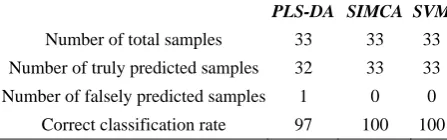
Table 3. Performance of three supervised pattern recognition techniques in the classification of mineral water samples
PLS-DA SIMCA SVM
Number of total samples 33 33 33
Number of truly predicted samples 32 33 33
Number of falsely predicted samples 1 0 0
Correct classification rate 97 100 100
of the 33 water classes both samples were correctly assigned (correct classification rate of 97%). One test set sample of class 30 was partially misclassified as that sample was assigned to two classes: one correct and another wrong. These results indicate a presumably high classification power of the developed method.
SIMCA
SIMCA, a supervised learning technique, was used to create a PCA model for each class with which unknowns could be predicted. The optimum number of PCs used for each class was determined by cross validation. A PCA model for each class was constructed with a different number of optimum PCs. All training data and test data were correctly classified with this SIMCA model and the algorithm achieves a correct classification rate of 100% (Table 3).
Least Squares Support Vector Machine
Similar to other multivariate statistical models, the performances of LS-SVM for classification depend on the combination of several parameters, such as kernel function and the corresponding kernel parameters. For classification tasks, a commonly used kernel function is the radial basis function (RBF) because of its good general performance and a few parameters. Thus γ (the relative weight of the regression error) and σ2 (the
kernel parameter of the RBF kernel) need to be optimized. To determine the optimal parameters, a grid search was performed based on leave-one-out cross validation on the original training set for all parameter combinations of γ and σ2 from 0.01 to 100. No samples were wrong identified for all varieties of mineral waters and a correct classification rate of 100% was achieved (Table 3).
References
1. Güler C. Evaluation of maximum contaminant levels in Turkish bottled drinking waters utilizing parameters reported on manufacturer’s labeling and government-issued production licenses. J. Food Compos. Anal. 20: 262-272 (2007).
2. Güler C. Characterization of Turkish bottled waters using pattern recognition methods. Chemometr. Intell. Lab. Syst.
86: 86-94 (2007).
3. Versari A., Parpinello J.P., and Galassi S. Chemometrics survey of Italian bottled mineral waters by means of their labeled physico-chemical and chemical composition. J. Food Compos. Anal.15: 251-264 (2002).
4. Saleh M.A., Ewane E., Jones J., and Wilson B.L. Chemical evaluation of commercial bottled drinking water from Egypt. J. Food Compos. Anal.14: 127-152 (2001). 5. Warburton D.W., Dodds K.L., Burke R., and Johnston
water sold in Canada between 1981 and 1989. Can. J. Microbiol.38: 12-19 (1992).
6. Garzon P., and Eisenberg M.J. Variation in the mineral content of commercially available bottled waters: Implications for health and disease. Am. J. Med.105: 125-130 (1998).
7. Warburton D.W., Dodds K.L., Burke R., Johnston M.A., and Laffey P.J. A review of the microbiological quality of bottled water sold in Canada between 1981 and 1989.
Can. J. Microbiol.38: 12-19(1992).
8. Fiket Ž., Roje V., Mikac N., and Kniewald G. Determination of arsenic and other trace elements in bottled waters by high resolution inductively coupled plasma mass spectrometry. Croat. Chem. Acta80: 91-100 (2007).
9. Martens H., and Naes T. Multivariate calibration. Wiley, Chichester, (1989).
10. Massart D., Vandeginste B., Buydens L., and De Jong S.
Handbook of Chemometrics and Qualimetrics. Elsevier, Amsterdam, (1998).
11. Brereton R. Chemometrics, Data Analysis for the Laboratory and Chemical Plant. Wiley, Chichester, (2003).
12. Johnson D.E. Applied Multivariate Methods for Data Analysts. Duxbury Press, Pacific Grove, (1998).
13. Reyment R., and Jöreskog K.G. Applied Factor Analysis in the Natural Sciences. Cambridge University Press, London, (1993).
14. Marengo E., Gennaro M.C., Giocosa D., Abrigo C., Saini G., and Avignone, M.T. How chemometrics can helpfully assist in evaluating environmental data. Lagoon water.
Anal. Chim. Acta317: 53-63 (1995).
15. Krzanowski W.J. Recent trends and developments incomputational multivariate analysis, Stat. Comput., 7: 87-99 (1997).
16. Brodnjak-Vončina D., Dobčnik D., Novič M., and Zupan J. Chemometrics characterisation of the quality of river water. Anal. Chim. Acta462: 87-100 (2002).
17. Yekdeli-Kermanshahi K., Tabaraki R., Karimi H., Nikorazm M., and Abbasi S. Classification of Iranian bottled waters as indicated by manufacturer’s labellings.
Food Chem.120: 1218-1223 (2010).
18. Lourenço C., Ribeiro L., and Cruz, J. Classification of natural mineral and spring bottled waters of Portugal using principal component analysis. J. Geochem. Explor. 107: 362–372 (2010).
19. Kraic F., Mocák J., Fiket Ž., and Kniewald G. ICP MS analysis and classification of potable, spring, and mineral waters. Chem. Papers62: 445-450 (2008).
20. Sharaf M.A., Illman D.L., and Kowalski B.R.
Chemometrics. John Wiley, New York, (1986).
21. Beebe K.R., Pell, R.J., and Seasholtz, M.B.
Chemometrics: A Pratical Guide. Wiley, New York, (1998).
22. Wold S. Pattern recognition by means of disjoint principal components models. Pattern Recogn.8: 127-139 (1976). 23. Flaten G.R., Grung B., and Kvalheim O.M. A method for
validation of reference sets in SIMCA modeling. Chemom. Intell. Lab. Syst.72: 101-109 (2004).
24. Barker M., and Rayens W. Partial least squares for discrimination. J. Chemom.17: 166-173 (2003).
25. Geladi P., and Kowalski B.R. Partial least-squares: A tutorial. Anal. Chim. Acta185: 1-17 (1986).
26. Tominaga Y. Comparative study of class data analysis with PCA-LDA, SIMCA, PLS, ANNs and k-NN.
Chemom. Intell. Lab. Syst.49: 105-115 (1999).
27. Cortes C., and Vapnik V. Support vector networks. Mach. Learn.20: 273-297 (1995).
28. Vapnik V. Statistical Learning Theory. John Wiley, New York, (1998).
29. Suykens J.A.K., and Vandewalle J. Least squares support vector machine classifiers. Neural Process. Lett.9: 293-300. (1999).
30. Suykens J.A.K., Van Gestel T., De Brabanter J., De Moora B., and Vandewalle, J. Least-Squares Support Vector Machines. World Scientifics, Singapore (2002). 31. Zou T., Dou Y., Mi H., Zou J., and Ren Y. Support vector
regression for determination of component of compound oxytetracycline powder on near-infrared spectroscopy.
Anal. Biochem.355: 1-7 (2006).
32. Ke Y., and Yiyu C. Discriminating the genuineness of Chinese medicines using least squares support vector machines. Chinese J. Anal. Chem.34: 561-564 (2006). 33. Borin A., Ferrao M.F., Mello C., Maretto D.A., and Poppi
R.J. Least-squares support vector machines and near infrared spectroscopy for quantification of common adulterants in powdered milk. Anal. Chim. Acta579: 25-32 (2006).