Boundary layer flow beneath a uniform free stream permeable continuous moving surface in a nanofluid

Address correspondence to: Ioan Pop, Department of Mathematics, Babes-Bolyai University, 400048 Cluj-Napoca, Romania

E-mail: [email protected]

1.

Introduction

Many industrial processes involve the transfer of heat by means of a flowing fluid in either the laminar or turbulent regime as well as flowing or stagnant boiling fluids. The processes cover a large range of temperatures and pressures. Many of these applications would benefit from a decrease in the thermal resistance of the heat transfer fluids. This situation would lead to smaller heat transfer systems with lower capital cost and improved energy efficiencies. An innovative technique, which uses a mixture of nanoparticles and a base fluid, was first introduced by Choi [1] to develop advanced heat transfer fluids with substantially higher conductivities. The resulting mixture of the base fluid and nanoparticles having unique physical and chemical properties is referred

to as a nanofluid. Flow and heat in a nanofluid over a stretching/shrinking sheet have become a hot topic and have attracted the interest of many researchers recently. The interest in this field has been stimulated due to its applications in industrial processes such as in power generation, chemical processes, and heating or cooling processes. The solid nanoparticles have been suspended into the base fluid which has poor heat transfer properties in order to increase its thermal conductivity. Choi et al. [2] reported that the thermal conductivity of the base fluids increases up to approximately two times with the addition of a small amount (less than 1% by volume fraction) of nanoparticles to the base fluids. A good literature on convective flow and applications of nanofluids were done in the books by Das et al. [3], and Nield and Bejan [4], and in the review papers by Buongiorno [5-7], Kakaç and

Boundary layer flow beneath a uniform free stream permeable continuous

moving surface in a nanofluid

Ioan Pop

, Sarkhosh Seddighi

, Norfifah Bachok

, Fudziah Ismail

1

Department of Mathematics, Babes-Bolyai University, 400048 Cluj-Napoca, Romania

2_{Department of Mathematics and Institute for Mathematical Research, University Putra Malaysia, 43400 UPM Serdang, Selangor, Malaysia} 3_{Department of Mathematics, Science and Research Branch, Islamic Azad University, Bushehr Branch, Bushehr, Iran}

4_{Nuclear Science Research School, Nuclear Science and Technology Research Institute (NSTRI),} P.O. Box 14395-836, Tehran, Iran

Journal of Heat and Mass Transfer Research

Journal homepage: http://jhmtr.journals.semnan.ac.ir

A B S T R A C T

The main purpose of this paper is to introduce a boundary layer analysis for the fluid flow and heat transfer characteristics of an incompressible nanofluid flowing over a permeable isothermal surface moving continuously. The resulting system of non-linear ordinary differential equations is solved numerically using the fifth–order Runge–Kutta method with shooting techniques using Matlab and Maple softwares. Numerical results are obtained for the velocity, temperature, and concentration distributions, as well as the friction factor, local Nusselt number, and local Sherwood number for several values of the parameters, namely the velocity ratio parameter, suction/injection parameter, and nanofluid parameters. The obtained results are presented graphically in tabular forms and the physical aspects of the problem are discussed.

© 2014 Published by Semnan University Press. All rights reserved.

PAPER INFO

History: Received 5 February 2014

Received in revised form 4 April 2014

Accepted 8 April 2014

Keywords

:

Pramuanjaroenkij [8], Wong and Leon [9], Saidur et al. [10], Wen et al. [11], Mahian et al. [12], and many others. The flow induced by a moving boundary is important in the study of extrusion processes and is a subject of considerable interest in the contemporary literature (Fang et al. [13]). For example, materials which are manufactured by extrusion processes as well as heat-treated materials travelling between a feed roll and a wind-up roll or on conveyor-belts possess the characteristics of stretching/shrinking surfaces. Polymer sheets and filaments are also manufactured by continuous extrusion from a die to a windup roller which is located a finite distance away (Sparrow and Abraham [14]). For both impermeable and permeable shrinking sheets, multiple solutions were discovered (Liao and Pop [15]). Most of these solutions are based on the boundary layer assumption and therefore do not constitute exact solutions of the Navier–Stokes equations (Wang [16]). The influence of thermal radiation on boundary layer flow over a shrinking sheet in a nanofluid has been studied by Zaimi et al. [17]. The partial differential equations are transformed to the ODE and are solved by shooting alongside with sixth order of Runge-Kutta integration technique. It is observed that radiation has dominant effect on the heat transfer and the mass transfer rates. In general, suction tends to increase the skin friction and heat transfer coefficients, whereas injection acts in the opposite manner. Bachok et al. [18, 19] have studied the boundary layer flow over a stretching/shrinking surface in a nanofluid. Finally, we mention the paper by Ibrahim et al. [20] on the MHD stagnation point flow and heat transfer due to nanofluid towards a stretching sheet.

In this study, five different types of nanoparticles, Silver Ag, Copper Cu, Copper Oxide CuO, Titania

TiO

flow over a permeable continuous moving surface with suction and injection. The governing boundary layer equations have been transformed to a two-point boundary value problem using similarity variables. These have been numerically solved using fourth order Runge–Kutta method with shooting technique. The effects of governing parameters on fluid velocity, temperature, and particle concentration have been discussed.

2.

Mathematical formulation

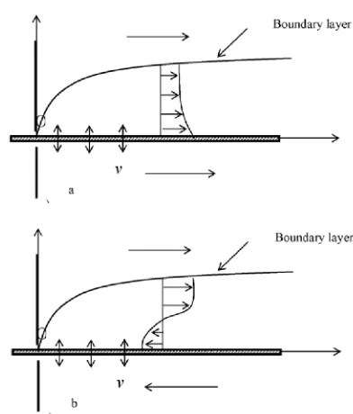
Consider a steady flow of a nanofluid in the region 0

y past a moving semi-infinite permeable flat plate, as shown in Fig. 1, where x and y are the Cartesian coordinates measured along the plate and are normal to it, respectively. It is assumed that the plate moves into or out

of the origin at the uniform speedU, where U is the constant velocity of the external (inviscid) flow and  is the constant moving parameter. 0 corresponds to the downstream movement of the plate from the origin and

0

 corresponds to the plate moving into the origin (opposing flow). It is also assumed that the mass flux velocity isv_w( )x , where v_w( )x 0 corresponds to the suction and v_w( )x 0 corresponds to the injection or withdrawal of the fluid, respectively. Further, we assume that the uniform temperature and the uniform nanofluid volume fraction at the surface of the plate are T_w and

,

w

C while the uniform temperature and the uniform nanofluid volume fraction far from the surface of the plate are T_ and C_, respectively (see Kuznetsov and Nield [21]). Under these assumptions, the basic nanofluid conservation equations are (Buongiorno [5-7] and Tivari and Das [22]):

0

u v

x y

 

 

  (1)

2 2

2 2

1 nf

nf nf

u u p u u

u v

x y x x y



 

 

    

      

   _  _ (2)

2 2

2 2

1 nf

nf nf

v v p v v

u v

x y y x y



 

 

    

      

   _  _ (3)

2 2 2 2 2 2 nf B T

T T T T

u v

x y x y

C T C T

D

x x y y

D T T

T x y

                _  _                         _{ }        _{ }        _{   }            (4) 2 2 2 2 2 2 2 2 B T

C C C C

u v D

x y x y

D T T

T x y

             _  _               (5)

boundary conditions of these equations are:

, , ,

at 0

, 0, ,

as

w w w

w

u u U v v T T

C C y

u U U v T T

C C y

                 (6)

C is the nanoparticle volume fraction, p is the pressure,

f

 is the density of the nanofluid, D_B is the Brownian diffusion coefficient and D_T is the thermophoretic diffusion coefficient, (C) /(_p C)_f , where (C)_f is the heat capacity of the fluid and (C)_p is the effective heat capacity of the nanoparticle material, respectively.

n f

 is the effective thermal diffusivity of the nanofluid,

n f

 is its effective viscosity of the nanofluid, and _{n f} is its effective density of the nanofluid, which are given by (Khanafer et al. [23] or Oztop and Abu-Nada [24]):

f nf

nf _2.5 nf

p nf

p nf p f p s

s f f s

nf

f s f f s

, ,

( C ) (1- )

( ) (1 ) ( C ) ( C )

( 2 ) 2 ( )

( 2 ) ( )

k

C

k k k k

k

k k k k k

                        (7)

where _f is the dynamic viscosity of the base fluid being proposed by Brinkman [25], k_{n f} is the thermal conductivity of the nanofluid, k_f and k_s are the thermal conductivities of the base fluid and of the solid particles, respectively. (C_{p n f}) is the heat capacitance of the nanofluid. Strictly, expressions (7) are restricted to spherical (or near spherical) nanoparticles with other expressions being required for other shapes of nanoparticles.

We define now the following boundary layer variables

1/ 2

1/ 2

2

, Re , ,

Re , , ,

, ,

w w

w w

w w

f

x y u

x y u

L L U

u v

v

v u v

U U U

p p T T C C

p h

T T C C

U                      (8)

whereL is the characteristic length of the plate and ReU L/_f is the Reynolds number. Substituting Eq. (9) for Eqs. (1) to (5) and using the boundary layer approximation in which Re1, we obtain the following dimensionless boundary layer equations for the problem under consideration: 0 u v x y       (9) 2 2 nf f nf

u u u

u v

x y y

  

  

 

   (10)

2 2 2 nf f T B f u v

x y y

h D

D

y y T y

                   _{ }         _{ }    _ _    (11) 2 2 2 2 B T f f

h h D h D

u v

x y y T y

   _            (12)

with the new boundary conditions as follows:

, ( ), 1, 1 at 0

1, 0, 0 as

w w

u u v v x h y

u h y

 



     

     (13)

We look for a similarity solution to Eqs. (9-12) along with the boundary conditions (13) of the following form (see Weidman et al. [26]):

2 ( ), ( ), ( ), / 2

x f h h

y x            (14)

where is the stream function which is defined in the usual form as u  /yandv  /x. Thus, we have:

'( ), (1 / 2 ( ) '( )

u f  v  x f_   f  _ (15)

where primes denote differentiation with respect to . In order that Eqs. (9-12) have similarity solutions; it is necessary that v_w( )x has the following form:

0 ( ) (1 / 2 )

w

v x   x f (16)

where f₀ is the constant mass flux parameter with f₀0 for suction and f₀0 for injection, respectively.

Substituting variables (14) for Eqs. (9) to (12), we obtain the following ordinary (similarity) differential equations:

2.5 1

''' '' 0 (1 ) (1 _s/ _f)

f f f

      

   (17)

2.5

2 / 1

''

Pr (1 ) 1 ( ) / ( )

' ' ' ' 0

nf f

p s p f

k k

C C

f Nb h Nt

            _   _     (18)

'' ' Nt '' 0 h Le f h

Nb

   (19)

and the boundary conditions (13) become:

0

(0) , '(0) , (0) 1, (0) 1 '( ) 1, ( ) 0, ( ) 0 as

f f f h

here Pr is the Prandtl number,Le is the Lewis number, Nb is the Bronian parameter, and Nt is the thermophoresis parameter, which are defined as:

( )

, , ,

( )

f f B w

f B f

T w

f

D C C

Pr Le Nb

D

D T T

Nt T                 (21)

The quantities of practical interest in this study are the skin friction coefficient C_f , the local Nusselt number

x

Nu , and the local Sherwood number Sh_x, which are defined as:

2, _{( )},

( ) w w f x f w f m x B w

x x q

C Nu

k T T

U

x q Sh

D C C

         (22)

where _w, qw, and qm are the surface shear stress, the

surface heat flux, and the surface mass flux would be:

0 0

0

, ,

w nf w nf

y y m B y u T q k y y C q D y           _{ }   _{ }                (23)

Using variables (8) and (14), we obtain:

1/ 2

2.5

1/ 2

1/ 2

1

(2Re ) ''(0),

(1 ) (2 / Re ) '(0),

(2 / Re ) '(0)

x f nf x x f x x C f k Nu k Sh h         (24)

where Re_xU x/_f is the local Reynolds number. It is worth mentioning to this end that for  0(pure viscous fluid), Eq. (17) with the corresponding boundary conditions (20) for f( ) reduces to Eq. (4a) with the boundary conditions (4b,c,d) from the paper by Wedman et al. [26].

3.

Results and discussion

Numerical solutions to the nonlinear ordinary differential equations (17-19) with the boundary conditions (20) were obtained using the fifth–order Runge–Kutta [27] with the shooting technique. We find

Figure 1. Physical model and coordinate system: a) flat plate moving out of the origin; b) flat plate moving into

the origin

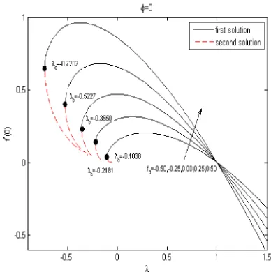
the missing slopes f''(0) and '(0), for some values of the governing parameters, namely, the nanoparticle volume fraction , the moving parameter , and the suction/injection parameter f₀ using the Maple and Matlab softwares. Five types of nanoparticles were considered, namely, Ag, Cu, CuO,TiO , and ₂ Al O . 2 3 Following Oztop and Abu-Nada [24], the value of the Prandtl number Pr is taken as 6.2 (for water) and the values of the volume fraction parameter  is from 0 to 0.2 ( 00.20) in which  0 corresponds to the pure (Newtonian) fluid. It is worth mentioning that we have used data related to thermophysical properties of the fluid and nanoparticles as listed in table 1 to compute each case of the nanofluid. The numerical results are summarized in Table 2 and Figs. 2 to 16.

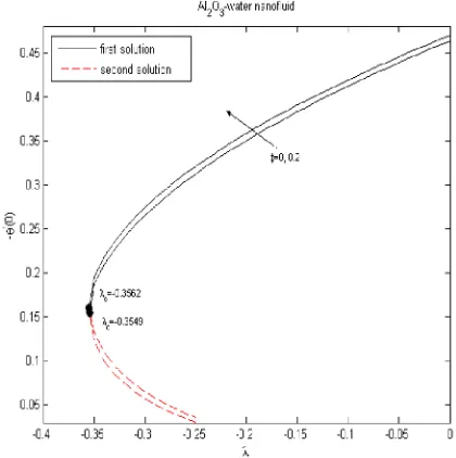
Figs. (2) to (7) show the variation of f''(0) (skin-friction coefficient) with respect to  for Ag, Cu, CuO,

2

TiO , and Al O - water nanofluids and different values _{2 3} of f₀ when Nb0.3, Nt0.1, Le1, Pr0.1, and

0.1

  . It is seen that the solution is unique when 0. There are two solutions (upper and lower branches) when

0

c

  (opposite flow), and no solution when 0

c

the solution exists. The values of f''(0) are positive when 1

 , and they become negative when the value of 

exceeds 1, for all values of the suction/injection parameter 0

f . Physically, the positive value of f''(0) means that the fluid exerts a drag force on the plate, and the negative value means the opposite. The zero value of f''(0)when

1

 does not mean separation, but it corresponds to the equal velocity of the plate and the free stream. A comparison of the obtained values _c for several values of f₀ with those reported by Weidman et al. [26] is given in Table 2. It is seen that the results are in a very good agreement so that we are confident that the present results are accurate.

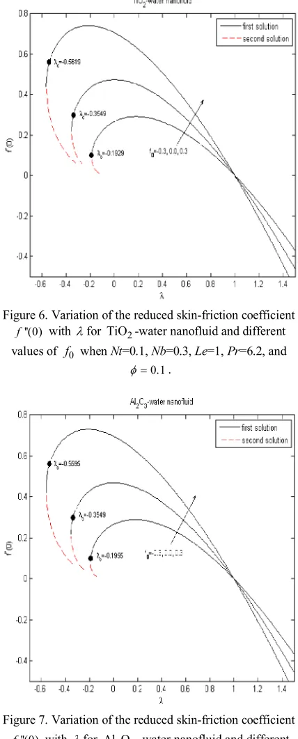
Fig. (8) shows the variation of the reduced skin-friction coefficient f''(0) with respect to  for Ag,

2

Cu, CuO, TiO , and Al O -water nanoparticles when 2 3 0.1,

Nb0.3, Nt0.1, Le1, Pr f00, and  0.1. The skin-friction f''(0) increases when the nonoparticles have the order ofAgCuCuOTiO₂Al O_{2 3}. As it is clear from Fig. (7), the difference between two nonoparticles TiO and ₂ Al O is so less compared to _{2 3} other particles.

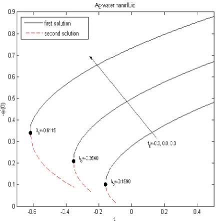
Figs. (9) and (10) show the variation of '(0) with respect to  for Ag- water and Al O - water nanofluids _{2 3} and different values of the f₀ when

0.1,

Nb0.3, Nt0.1, Le1, Pr f₀0,and  0.1. It is seen that the solution is unique when0, while dual solutions are found to exist when 0¸ i.e. when the plate and the free stream move in the opposite directions. The values of - h'(0) are positive for all values (positive or negative) of  and for all values of the suction/injection parameter f₀.

The variation of f''(0) and '(0) with respect to 

for Ag and Al O - water nanoparticles and different _{2 3} values of nanoparticle volume fraction (0 and 0.2) when Nb0.3, Nt0.0, Le1, Pr0.1, and f₀0 (impermeable plate) has been shown in Figs. (11) to (14). The values of f''(0)are positive when1, and they become negative when the value of exceeds 1, for both values of the parameter  considered. The values of

'(0)



 are positive for all values of and for both values of nanoparticle volume fraction . The values of f''(0) and '(0) increase when the variable increases from 0

Figure 2. Variation of the reduced skin-friction coefficient ''(0)

f with for  0 and different values of f₀ when Nt = 0.1, Nb=0.3, Le=1, and Pr=6.2.

Figure 3. Variation of the reduced skin-friction coefficient ''(0)

f with for Ag-water nanofluid and different values of f₀ when Nt=0.1, Nb=0.3, Le=1, Pr=6.2, and 0.1.

to 0.2. The variation of



  ) is very fiddling.

Figs. (2) to (14) also show that for a particular value of 0

f , the solution exists up to the certain critical value of 0

c

Figure 4. Variation of the reduced skin-friction coefficient ''(0)

f with for Cu-water nanofluid and different values of f₀ when Nt=0.1, Nb=0.3, Le=1, Pr=6.2, and 0.1.

Figure 5. Variation of the reduced skin-friction coefficient ''(0)

f with for CuO-water nanofluid and different values of f₀ when Nt=0.1, Nb=0.3, Le=1, Pr=6.2, and

0.1

 .

solution cannot be obtained. The boundary layer separates from the surface at _c0. Based on our computations, the critical values of _care presented in Table (2), which show that for all nanoparticles considered, the values of _c increase as f₀ increases.

Figure 6. Variation of the reduced skin-friction coefficient ''(0)

f with for TiO -water nanofluid and different ₂ values of f₀ when Nt=0.1, Nb=0.3, Le=1, Pr=6.2, and

0.1

 .

Figure 7. Variation of the reduced skin-friction coefficient ''(0)

f with for Al O_{2 3}-water nanofluid and different values of f₀ when Nt=0.1, Nb=0.3, Le=1, Pr=6.2, and

0.1

 .

Figure 8. Variation of the reduced skin-friction coefficient ''(0)

f with  for Ag, Cu, CuO, TiO ,Al O -water _{2 2 3} nanofluid when Nt=0.1, Nb=0.3, Le=1, Pr=6.2, and

0.1

 .

Figure 9. Variation of '(0) with  for Ag -water nanofluid when Nt= 0.1, Nb=0.3, Le=1, Pr=6.2, and

0.1

 .

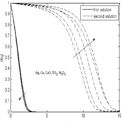
Finally, Figs. (15) and (16) present the velocity '( )

f  and the temperature  ( ) profiles for Ag, Cu, CuO, TiO , and ₂ Al O - water nanofluids when_{2 3}

Figure 10. Variation of '(0) with for Al O -water _{2 3} nanofluid when Nt=0.1, Nb=0.3, Le=1, Pr=6.2, and

0.1

 .

Figure 11. Variation of the reduced skin-friction coefficient f''(0) with for Ag -water nanofluid and

different values of  when Nt=0.1, Nb=0.3, Le=1, Pr=6.2, and f₀0.

0.1,

Nb0.3, Nt0.1, Le1, Pr f00, 0.1, and 0.3

Figure 12. Variation of the reduced skin-friction coefficient f''(0) with forAl O -water nanofluid and _{2 3}

different values of  when Nt= 0.1, Nb=0.3, Le=1, Pr= 6.2, and f₀0.

Figure 13. Variation of '(0) with for Ag -water nanofluid and different values of  when Nt=0.1, Nb=0.3,

Le=1, Pr=6.2, and f₀0.

boundary conditions equation (19). In these figures the solid lines and the dash lines are for the upper and lower branch solutions, respectively.

Figure 14. Variation of '(0) with for Al O -water _{2 3} nanofluid and different values of  when Nt=0.1, Nb=0.3,

Le=1, Pr=6.2, and f₀0.

Figure 15. Velocity profile for Ag, Cu, CuO, TiO ,Al O_{2 2 3} - water nanofluids when Nt=0.1, Nb=0.3, Le=1, Pr=6.2,

0.1

 , 0.1, and f₀0.

4. Conclusion

This paper have been theoretically the existence of dual similarity solutions in boundary layer flow over a moving

surface immersed in a nanofluid with suction and injection effects have been theoretically studied. The governing boundary layer equations were solved numerically using the fifth–order Runge–Kutta method with shooting Figure 16. Temperature profiles for Ag, Cu, CuO, TiO ,Al O - water nanofluids when Nt=0.1, Nb=0.3, Le=1, _{2 2 3}

Pr=6.2, 0.1,  0.1, and f₀0.

Table 1.Thermophysical properties of fluid and nanoparticles (Oztop and Abu-Nada [22])

Physical properties Fluid phase (water) Ag Cu CuO Al O2 3 TiO₂

( )

p

C J/kg K 4179 235 385 531.8 765 686.2

3

(kg/m )

 997.1 10500 8933 6320 3970 4250

(W /m K)

k 0.613 429 400 76.5 40 8.9538

Table 2. Comparison of the values of c for various f0 when  0(pure fluid)

0

f c c

Weidman et al. [24 ] Present

-0.50 -0.1035 -0.1035

-0.25 -0.2125 -0.2181

0.00 -0.3541 -0.3541

0.25 -0.5224 -0.5227

technique using the Matlab 12a software. Discussion were carried out for the effects of nanoparticle volume fraction , suction/injection parameterf₀, and the moving parameter  on the skin friction coefficient f''(0) and the local Nusselt number '(0). It was found that dual solutions exist when the plate and the free stream move in the opposite directions. It was also shown that introducing the suction increases the range of for which the solution exists, and in consequence delays the boundary layer separation, while it was found that the injection acts in the opposite manner.

Acknowledgements

The authors wish to express their thanks to the anonymous Reviewers for their valuable comments and suggestions. The financial supports received from the Ministry of Higher Education, Malaysia (Project codes: FRGS/1/2012/SG04/UPM/03/1) and the Research University Grant (RUGS) from the University Putra Malaysia are gratefully acknowledged.

Nomenclature

p

c

Specific heat capacity

f

C

skin friction coefficient

f

dimensionless stream function

k

thermal conductivity

x

Nu

local Nusselt number

Pr

Prandtl number

w

q

surface heat flux

x

Re

local Reynolds number

w

T

plate temperature

T

fluid temperature

T

ambient temperature

,

u v

velocity components along the and

directions, respectively

U

plate velocity

U

free stream velocity

, u v

Components of velocity

x y

Cartesian coordinates along and

normal to the surface, respectively

Greek letters



Thermal diffusivity



nanoparticle volume fraction



Dynamic viscosity



Kinematics viscosity



Density



Dimensionless temperature



velocity ratio parameter

w



surface shear stress



stream function



similarity variable

Subscript

s

solid

f

Fluid

nf

nanofluid



ambient condition

w

condition at the surface of the plate

Superscript

'

differentiation with respect to



References

[1]. S.U.S. Choi, Enhancing thermal conductivity of fluids with nanoparticles. In: Developments and Applications of Nonnewtonian Flows (D. A. Singer and H. P. Wang, Eds.), American Society of Mechanical Engineers, New York, NY, USA, 231, 99-105 (1995).

[2]. S.U.S Choi, Z.G. Zhang, W. Yu, F.E. Lockwood, E.A. Grulke, Anomalously thermal conductivity enhancement in nanotube suspensions, Appl. Phys. Lett., 79, 2252-2254 (2001).

[3]. S.K. Das, S.U.S. Choi, W. Yu, T. Pradeep, Nanofluids: Science and Technology, Wiley, New Jersey, (2007). [4]. D.A. Nield, A. Bejan, Convection in Porous Media (4th

edition), Springer, New York, (2013).

[5]. J.Buongiorno, Convective transport in nanofluids., ASME J. Heat Transfer, 128, 240-250 (2006).

[6]. M. J. Maghrebi · M. Nazari · T. Armaghani, Forced Convection Heat Transfer of Nanofluids in a Porous Channel, Transp Porous Med, 93, 401–413 (2012). [7]. T. Armaghani, M.J. Maghrebi, A.J. Chamkha, M, Nazari,

Effects of Particle Migration on Nanofluid Forced Convection Heat Transfer in a Local Thermal Non-Equilibrium Porous Channel, 3, 51-59 (2014).

[8]. S. Kakaç, A. Pramuanjaroenkij, Review of convective heat transfer enhancement with nanofluids, Int. J. Heat Mass Transfer, 52, 3187-3196 (2009).

[9]. K.V. Wong, O.D. Leon, Applications of nanofluids: current and future, Adv. Mech. Eng., Article ID 519659, 1-11 (2010).

[10].R. Saidur, K.Y. Leong, H.A. Mohammad, A review on applications and challenges of nanofluids, Renewable and Sustainable Energy Reviews, 15, 1646-1668 (2011). [11].D. Wen, G. Lin, S. Vafai, K. Zhang, Review of nanofluids

for heat transfer applications, Particuology, 7, 141-150 (2011).

[12].O. Mahian, A. Kianifar, S.A. Kalogirou, I. Pop, S. Wongwises, A review of the applications of nanofluids in solar energy, Int. J. Heat Mass Transfer, 57, 582–594 (2013).

[13].T. Fang, S. Yao, J. Zhang, A. Aziz, Viscous flow over a shrinking sheet with a second order slip flow model, Commun. Nonlinear Sci. Numer. Simulat, 15, 1831–1842 (2010).

[15].S.J. Liao, I. Pop, A new branch of solutions of boundary-layer flows over a stretching flat plate, Int. J. Heat Mass Transfer, 49, 2529–2539 (2005).

[16].C.Y. Wang, Exact solutions of the steady state Navier– Stokes equations, Ann. Rev. Fluid Mech., 23, 159–177 (1991).

[17].K. Zaimi, A. Ishak, I. Pop, Boundary layer flow and heat transfer past a permeable shrinking sheet in a nanofluid with radiation effect, Adv. Mech. Eng., Article ID 340354, 1-7 (2012).

[18].N. Bachok, A. Ishak, I. Pop, The boundary layers of an unsteady stagnation-point flow in a nanofluid, Int. J. Heat Mass Transfer, 55, 6499–6505 (2012).

[19].N. Bachok, A. Ishak, I. Pop, Boundary layer stagnation-point flow toward a stretching/shrinking sheet in a nanofluid, ASME J. Heat Transfer, 135 (Article ID 05450), 1-5 (2013).

[20].W. Ibrahim, B. Shankar, M.M. Nandeppanavar, MHD stagnation point flow and heat transfer due to nanofluid towards a stretching sheet, Int. J. Heat and Mass Transfer, 56, 1–9 (2013).

[21].A.V. Kuznetsov, D.A. Nield, Natural convective boundary-layer flow of a nanofluid past a vertical plate, Int. J. Thermal Sci., 49, 243–247 (2010).

[22].R.K. Tiwari, M.K. Das, Heat transfer augmentation in a two-sided lid-driven differentially heated square cavity utilizing nanofluids, Int. J. Heat Mass Transfer , 50, 2002-2018 (2007).

[23].K. Khanafer, K. Vafai, M. Lightstone, Buoyancy-driven heat transfer enhancement in a two-dimensional enclosure utilizing nanofluids, Int. J. Heat Mass Transfer, 46, 3639– 3653 (2003).

[24].H.F. Oztop, E. Abu-Nada, Numerical study of natural convection in partially heated rectangular enclosures filled with nanofluids, Int. J. Heat Fluid Flow, 29, 1326–1336 (2008).

[25].H.C. Brinkman, The viscosity of concentrated suspensions and solution, J. Chem. Phys., 20, 571-581 (1952). [26].P.D. Weidman, D.G. Kubitschek, A.M.J. Davis, The

effect of transpiration on self-similar boundary layer flow over moving surfaces, Int. J. Eng. Sci., 44, 730-737 (2006). [27].S. Seddighi Chaharborja, S.M. Sadat Kiai, M.R. Abu Bakar, I. Ziaeian, I. Fudziah, A new impulsional potential for a Paul ion trap, Int. J. Mass Spectrom, 309, 63– 69 (2012).

[28].A.V. Kuznetsov, D.A. Nield, Natural convective boundary-layer flow of a nanofluid past a vertical plate, Int. J. Thermal Sci., 49, 243–247 (2010).

[29].R.K. Tiwari, M.K. Das, Heat transfer augmentation in a two-sided lid-driven differentially heated square cavity utilizing nanofluids, Int. J. Heat Mass Transfer , 50, 2002-2018 (2007).

[30].K. Khanafer, K. Vafai, M. Lightstone, Buoyancy-driven heat transfer enhancement in a two-dimensional enclosure utilizing nanofluids, Int. J. Heat Mass Transfer, 46, 3639– 3653 (2003).

[31].H.F. Oztop, E. Abu-Nada, Numerical study of natural convection in partially heated rectangular enclosures filled with nanofluids, Int. J. Heat Fluid Flow, 29, 1326–1336 (2008).

[32].H.C. Brinkman, The viscosity of concentrated suspensions and solution, J. Chem. Phys., 20, 571-581 (1952). [33].P.D. Weidman, D.G. Kubitschek, A.M.J. Davis, The