Please cite this article in press as: Seid A. Multistate transition modeling: An application using hypertension data. J Biostat Epidemiol. 2016;
J Biostat Epidemiol. 2016; 2(2): 81-7.
Original Article
Multistate transition modeling: An application using hypertension data
Awol Seid1*
1
Department of Statistics, College of Computing and Informatics, Haramaya University, Dire Dawa, Ethiopia
ARTICLE INFO ABSTRACT
Received 03.10.2015 Revised 23.03.2016 Accepted 16.05.2016 Published 30.06.2016
Background & Aim: Multistate models are systems of multivariate survival data where individuals
move through a series of distinct states following certain paths of possible transitions. Such models provide a relevant tool for studying observations of a continuous time process at arbitrary times. The aim of this study was to model the transitions from a healthy (hypertension free) state to an illness (hypertension) state of a hypertensive patient under treatment.
Methods & Materials: In this article, the application of multistate modeling using hypertension
data is demonstrated. Hospital data were obtained for a cohort of 353 patients from Jimma University Hospital, Ethiopia.
Results: Three states of the Markov process are defined based on the WHO guideline of high blood
pressure, state 1 (BP < 140/90 mmHg), state 2 (BP ≥ 140/90 mmHg) and state 3 (dropout). The first state is termed as a healthy state, the second an illness state and the third one is an absorbing state. Initially, the state transition intensities and state occupation probabilities are estimated with no covariate. Then, the effect of gender and family history of hypertension on the state transition intensities are evaluated separately and jointly using proportional intensities model.
Conclusion: The study indicates that gender has a significant effect on the transition intensities but
not family history of hypertension.
Key words: Hypertension; Multistate modeling; Markov process
Introduction1
A multistate Markov model is a stochastic process in which subjects occupy one of a set of discrete states at any time. This model is convenient for describing repeated longitudinal events (stages) of the course of chronic diseases. In such cases, a patient may advance into or recover from adjacent disease stage which is called “transient” state or a patient at any disease stage may move to a state from which further transitions cannot occur called an “absorbing” state, often death or dropout.
This study demonstrates the application of multistate transition modeling using hypertension data. Hypertension is a chronic medical condition
* Corresponding Author: Awol Seid, Postal Address: Department of Statistics, College of Computing and Informatics, Haramaya University, Dire Dawa, Ethiopia. Email: [email protected]
in which the blood pressure in the arteries is elevated which requires the heart to work harder than normal to circulate blood through the blood vessels (1). As it is known, blood pressure is summarized by two measurements, systolic and diastolic, which depend on whether the heart muscle is contracting (systole) or relaxed between beats (diastole).
According to World Health Organization (2), high blood pressure is said to be present if it is persistently at or above 140/90 mmHg. Assuming that a hypertensive patient under anti-hypertensive treatment may recover from hypertension, three states of the Markov process are identified. These are defined as: state 1, blood pressure <140/90
mmHg; state 2, blood pressure ≥ 140/90 mmHg;
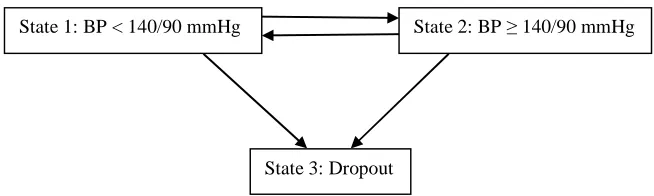
Figure 1.Paths between the states of the process. BP: Blood pressure
State 1 is categorized as a healthy state and state 2 is categorized an illness state. State 3, that is the dropout, is considered to be an absorbing state. The arrows in figure 1 show which transitions are possible between states. Transitions are permitted from health to illness, illness to dropout and health to dropout. Also recovery from illness to health is considered. Therefore, it is important to understand how the transitions among these states of hypertension take place and how the covariates influence these transitions.
Therefore, the multistate transition modeling of the hypertension states is used to predict the future clinical state and survival probability of a patient. Particularly, it is used to determine the conditional probability that a hypertensive patient can be in the next state of the disease given that the patient is in a known state of the disease, after a period of time; the conditional probability that a patient is staying in the same disease state until a specific time; and the probability that a patient survives for a specific time given the patient’s starting state of the disease. Following parts of this paper are organized as section 2 that describes the methods used, section 3 that presents the discussion of the main results of the study and finally, in section 4, conclusions are provided.
Methods
Description of the data
The data used in this paper is obtained from Jimma University Hospital, Ethiopia. All patients who were 18 years old or older and who had an anti-hypertensive treatment follow-up for a maximum of 18 months between September 2011 and January 2013 were included in the study. A total of 353 hypertensive patients
satisfied these inclusion criteria. Of these, 172 (48.73%) were females and the remaining 181 (51.27%) were males. In addition, 152 (43.06%) patients had and 201 (56.94%) did not have hypertension history in their family. Almost all of the patients were dropped out from the anti-hypertensive treatment while only 2 (0.57%) of the patients were following the treatment.
Multistate modeling
A multistate process, X(t), is a stochastic process with a finite state space of possible
transitions ξ = {1,2,…J} where J is the number of
states. The quantities of interest (state transition intensities and state occupation probabilities) can be calculated for complete data and also using estimators obtained from censored data when complete data is not known. It is useful to keep track of all the transitions an individual makes before ending in an absorbing state.
Let Tik represent the time of the kth transition
for individual i;i = 1, 2, …, n where Ti0 = 0 and
Tik = ∞ if the i
th
individual enters the absorbing state before the kth transition is made. Let Ci be
the right censoring time for the ith individual, Li
be the left truncation time for the ith individual
and Sik be the state occupied by the i
th
individual between times Ti,k-1 and Tik.
Let Ti = supk {Tik : Tik < ∞} be the time for the
last transition for individual i. The collection of all transition times and states occupied by individual i can be denoted as Ti = (Tik: k ≥ 1) and
si = (sik: k ≥ 1) , respectively. Let T∗ = min(Ti,Ci)
and let δi be an indicator of whether the i th
individual was never censored, δi = I(Ci > Ti).
The Nelson-Aalen estimator for the
integrated hazard matrix Λ and the
Aalen-Johansen estimator of the state occupation probability matrix of a Markov system are
State 1: BP < 140/90 mmHg State 2: BP ≥ 140/90 mmHg
presented in (3). The counting process and the number at risk for data subject to left truncation and right censoring are estimated as:
jj(t)=∑ ∑ I(Tik≤t, Ci≥Tik, Li<t, sik=j, si,k+1=j') (1)
and
jj(t)=∑ ∑ I(Ti,k-1<t≤Tik, Ci≥t, Li<t, sik=j) (2)
The Nelson-Aalen estimator of the
cumulative hazard is given by:
Λjj'(t)=
( () () )
dN (s), j ≠ j′
∑ Λ (t)( , j = j′
(3)
The Aalen-Johansen estimator of the
transition probability matrix of a Markov multistate system is obtained by product integration of Λjj', i.e.,
P(s,t)=∏,,-[I+ dΛ(u)] (4)
Where P(s,t) and Λ(t) are J×J matrices. Here
Λ={Λjj} which reduces to simple empirical
proportions for the complete data.
For Markov models, there will often be too little empirical basis for estimating freely varying transition intensities between all states for all subgroups, so that more parsimonious regression models are required [4]. The most frequently used regression models in event history analysis have a multiplicative structure with a baseline k→j transition intensity λkj0(t),
assumed common for all individuals (4). For an
individual, i, with time fixed covariates Zi(=Zim)
the transition intensity is then modeled as:
λ (t)=λ
kj0(t)exp(βzi) (5)
Where the effect of a covariate Zim is
described by factors of proportionality exp(βkjm).
In this equation, the baseline hazard may be completely unspecified as in the Cox proportional hazards model for survival data or it may be assumed to be piecewise constant leading to Poisson regression models (5, 6). Also this notation suggests that separate baseline hazards and regression coefficients are assumed for each possible transition. If that is the case, then the parameters may be estimated by fitting separate Cox or Poisson models for each transition (4). However, more parsimonious models may be obtained by assuming some baseline transition intensities proportional (7, 8) or by assuming some covariates to have the same effect on
several transitions (3). In addition, models where the proportional hazards assumption is relaxed may be considered. In the Poisson case this is simply an interaction between time and the covariate giving rise to non-proportionality whereas, for the Cox model, the less restrictive model is known as the stratified Cox model.
Results
Simple bi-direction transition model
The first step in a multistate model analysis is to set up the transition matrix that specifies which direct transitions are possible and assigns numbers to the transitions for future reference. Of the 353 patients, 254 stayed in state 1, 228 transited from state 1 to state 2 and 149 of them transited from state 1 to state 3. Also, 304 patients transited from state 2 to state 1, 810 stayed in state 2 and 202 transited from state 2 to state 3.
In multistate models of longitudinal data, usually a process is assumed to be Markovian, that is, the conditional probability distribution of future states depends only on the present state, not on the whole sequence of past events (9). Hence, all the analyses in this article are done under the Markov assumption that future evolution only depends on the current state. R software version 3.1.3 is used for the analysis using the msm package.
State transition intensities
The multistate model with three states labeled 1, 2, and 3 is shown in figure 1 above. At a time t, the individual is in state S(t). The next state to which the individual moves, and the time of the change, are governed by a set of transition intensities qkj(t) for each pair of states k and j, k,
jεξ. The intensity (hazard) represents the
instantaneous risk of moving from state k to state j. This intensity may depend on the time of the process t, or more generally a set of individual specific explanatory variables z. Therefore,
qkj(t)=lim△→P{S(t +△ t) = j|S(t) = k)}/△ t (6)
are then elements of a J×J matrix Q(t) whose rows sum to zero, so that the diagonal entries are defined by qkj(t)=-∑?(@>?@(A) and qkj(t) = 0 if a
constant in time (homogeneity assumption) or piecewise constant (10, 11, 12).
For the hypertension data, this transition intensity matrix together with the 95% confidence interval is estimated as shown in table 1. As can be seen from this table, patients in an illness state (state 2) are 2.684 (0.4890/0.1822) times as likely to transit to a healthy state (state 1) as dropout (state 3).
Table 1. Estimated baseline transition intensities
Transition states Baseline intensity
95% Confidence interval
State 1 to state 1 -1.0586 (-1.2960, -0.8647) State 1 to state 2 1.0586 ( 0.8647, 1.2960) State 2 to state 1 0.4890 ( 0.3933, 0.6080) State 2 to state 2 -0.6712 (-0.7894, -0.5707) State 2 to state 3 0.1822 ( 0.1638, 0.2028)
State occupation probabilities
The state occupation probability is the marginal probability that an individual being in state j at time t. Let pj(t) = P{S(t)=j} denote the
state j occupation probabilities t, jεξ. The process
has initial distribution. Where S(t) is the state occupied by an individual at time" here. Let pj(0)=P{S(0)=j};jεξ. Let B̂kj(s,t)=P{S(t)=j|S(s)=k}
be the transition probability to state j by time t given that the individual was in state k at time s. By fixing s and varying t, the future behavior of the multistate model can be predicted given the present at time s. For Markov models, these probabilities will depend only on the state at time s, not on what happened before (9). For incomplete data, the state transition probabilities are estimated as
pEj(t)=∑pE (0)pE (0, t) (7)
Where pE (0, t) is the (k,j) element of the
matrix pE (0,t) in equation (4) and pE (0) is the initial state occupation proportions for state k.
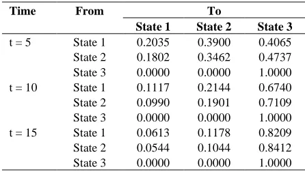
For the hypertension data, the estimated transition probability matrices within a given time t = 5, t = 10 and t = 15 months are presented in table 2.
Thus, a typical patient in a healthy state (state 1) has a probability of 0.8412 of being dropped-out (state 3) 15 months from now, a probability of 0.0613 being still in a healthy state (state 1), and a probability of 0.1178 of being with disease
(state 2), respectively.
Table 2. State occupation probabilities at t = 5, t = 10, and t = 15
Time From To
State 1 State 2 State 3
t = 5 State 1 0.2035 0.3900 0.4065 State 2 0.1802 0.3462 0.4737 State 3 0.0000 0.0000 1.0000 t = 10 State 1 0.1117 0.2144 0.6740 State 2 0.0990 0.1901 0.7109 State 3 0.0000 0.0000 1.0000 t = 15 State 1 0.0613 0.1178 0.8209 State 2 0.0544 0.1044 0.8412 State 3 0.0000 0.0000 1.0000
Mean Sojourn times and total length of stay
For processes with successive periods of recovery and relapse, it is better also to forecast the total time spent healthy or ill, before dropout. The total length of stay is an estimate of the forecasted total length of time spent in each
transient state j between two future time points t1
and t2. This defaults to the expected amount of
time spent in each state between the start of the process (time 0, the present time) and dropout or a specified future time. This is obtained as Ej= BHHI ?@(A)GA
J where k is the state at the start of
the process, which defaults to 1. For the above model, each patient is forecasted to spend a total of 3.4797 months in a healthy state (state 1) and 5.4879 months with disease (state 2).
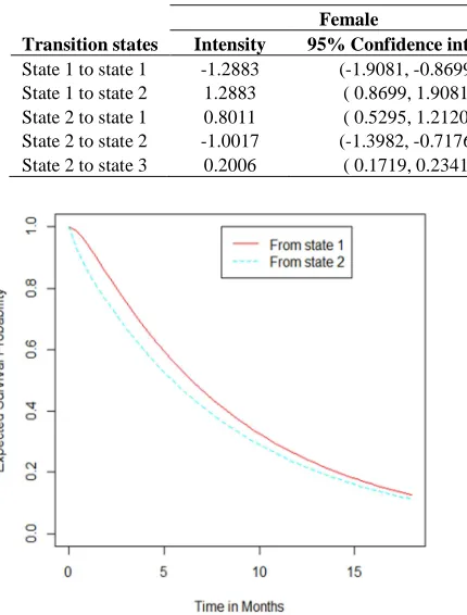
Another important use of multistate models is predicting the probability of survival for patients in different states of disease, for some time t in the future. This can be obtained directly from the transition probability matrix. Figure 2 is a plot of the expected probability of survival against time, from each transient state. The figure shows that the 18 months survival probability with an illness (state 2) is lower than the survival probability in the healthy status (state 1).
The effect of gender and family history of hypertension
Table 3. Estimated transition intensities by gender
Transition states
Gender
Female Male
Intensity 95% Confidence interval Intensity 95% Confidence interval
State 1 to state 1 -1.2883 (-1.9081, -0.8699) -0.9802 (-1.2623, -0.7611)
State 1 to state 2 1.2883 ( 0.8699, 1.9081) 0.9802 ( 0.7611, 1.2623)
State 2 to state 1 0.8011 ( 0.5295, 1.2120) 0.3286 ( 0.2484, 0.4345)
State 2 to state 2 -1.0017 (-1.3982, -0.7176) -0.4958 (-0.6017, -0.4085)
State 2 to state 3 0.2006 ( 0.1719, 0.2341) 0.1672 ( 0.1441, 0.1940)
Figure 2. Expected probability of survival
The result indicates that females in a healthy state (state 1) are 1.314 (1.2883/0.9802) times as likely to transit to an illness state (state 2) as those male patients. Also, females in an illness state (state 2) are 2.437 (0.8011/0.3286) and 1.199 (0.2006/0.1672) times as likely to transit to a healthy state (state 1) and a dropout state (state 3), respectively, as those male patients.
Again, to examine the effect of family history of hypertension, the proportional intensities model is fitted with family history alone (Table 4). Those patients who did not have family
history of hypertension were 0.804
(0.9655/1.2010) times as likely to transit from
state 1 to state 2 as compared to those patients who had family history. On the other hand, those patients who did not have family history of hypertension are 0.899 (0.4688/0.5212) and 1.115 (0.1914/0.1716) times as likely to transit from state 2 to state 1 and state 3, respectively, as those who had hypertension history in their family.
Next, to examine the joint effect of gender and family history of hypertension, the proportional intensities model was fitted with both of the covariates. The estimated intensities from this model are presented in table 5.
Also, the estimated hazard ratios
corresponding to each covariate effect of the proportional intensities model fitted with both of the covariates are presented in table 6. Regarding each possible transition, the only transition on which the effect of gender is significant at the 5% level of significance is the 2-1 transition. Hence, the intensity of moving from an illness state (state 2) to a healthy state (state 1) is 58% lower for male than female patients, given their hypertension family history.
Discussion
In this study, initially, a simple bidirectional model was fitted with no explanatory variable in order to examine the transition intensities, state occupation probabilities, mean Sojourn times, and total length of stay in a certain state after some time.
Table 4. Estimated transition intensities by family history of hypertension
Transition states
Family history of hypertension
No Yes
Intensity 95% Confidence interval Intensity 95% Confidence interval
State 1 to state 1 -0.9655 (-1.2480, -0.7470) -1.2010 (-1.6633, -0.8672)
State 1 to state 2 0.9655 ( 0.7470, 1.2480) 1.2010 ( 0.8672, 1.6633)
State 2 to state 1 0.4688 ( 0.3539, 0.6210) 0.5212 ( 0.3690, 0.7360)
State 2 to state 2 -0.6602 (-0.8107, -0.5377) -0.6927 (-0.9021, -0.5320)
Table 5. Estimated transition intensities by gender and family history of hypertension
Gender
Transition states
Family history of hypertension
No Yes
Intensity 95% Confidence interval
Intensity 95% Confidence interval
Female State 1 to state 1 -1.1459 (-1.7320, -0.7581) -1.4759 (-2.2307, -0.9764) State 1 to state 2 1.1459 ( 0.7581, 1.7320) 1.4759 ( 0.9152, 2.3798) State 2 to state 1 0.7358 ( 0.4762, 1.1368) 0.8815 ( 0.5290, 1.4689) State 2 to state 2 -0.9450 (-1.3304, -0.6713) -1.0713 (-1.5081, -0.7610) State 2 to state 3 0.2093 ( 0.1752, 0.2501) 0.1898 ( 0.1553, 0.2318) Male State 1 to state 1 -0.8858 (-1.1944, -0.6569) -1.1408 (-1.6675, -0.7805)
State 1 to state 2 0.8858 ( 0.6569, 1.1944) 1.1408 ( 0.7805, 1.6675) State 2 to state 1 0.3061 ( 0.2184, 0.4290) 0.3667 ( 0.2453, 0.5484) State 2 to state 2 -0.4811 (-0.6038, -0.3833) -0.5254 (-0.7009, -0.3939) State 2 to state 3 0.1750 ( 0.1464, 0.2092) 0.1587 ( 0.1313, 0.1918)
In multistate modeling, survival is defined as not entering the final absorbing state. Hence, it is essential to estimate the mean Sojourn time and total length of stay in a certain state. The mean Sojourn times describe the average period in a single stay in a state. For the hypertension data, the estimated mean Sojourn times in a healthy and illness states are 0.9446 months (95% CI 0.7716-1.1565) and 1.4898 months (95% CI 1.2668-1.7521), respectively. Thus, patients are more likely to stay in an illness state than a healthy state.
To examine the effect of gender and family history of hypertension, the proportional intensities model was first fitted with each covariate and then to determine the joint effect of both covariates, both covariates were fitted in the model. Of the two explanatory variables, it was revealed that only gender has a significant contribution on the rates of transition which is in line with another study (13) that showed that gender has an effect on the prevalence of hypertension.
In this study, the multistate modeling was applied to capture the dynamic stages of a hypertensive patient. The transition rates and
transition probabilities are estimated. Life history indicators such as state occupation times (Sojourn times) are estimated 0.94 and 1.49 months in a healthy and illness states, respectively. In addition, each patient spent a total of 3.48 months in a healthy state and 5.49 months with illness. The effects of gender and family history of hypertension were also examined and the result showed that gender has a significant contribution in only one of the possible transition. In particular, given the hypertension history, the hazard of transiting from an illness state to a healthy state for male patients is 0.42 times that of female patients.
Acknowledgments
Thanks to Jimma University for providing the hypertension data used in this study.
References
1. Awoke A, Awoke T, Alemu S, Megabiaw B.
Prevalence and associated factors of
hypertension among adults in Gondar, Northwest Ethiopia: a community based
Table 6. Estimated hazard ratios
Variable Hazard
ratio
95% Confidence interval
cross-sectional study. BMC Cardiovasc Disord 2012; 12: 113.
2. World Health Organization-international
society of hypertension guidelines for the management of hypertension. Guidelines Subcommittee. J Hypertens 1999; 17(2): 151-83.
3. Borgan O, Anderson PK, Gill RD, Keiding
N. Statistical models based on counting processes. Berlin, Germany: Springer; 1995.
4. Andersen PK, Keiding N. Multi-state models
for event history analysis. Stat Methods Med Res 2002; 11(2): 91-115.
5. Cox DR. Regression models and life-tables. J
R Stat Soc Series B 1972; 34(2): 187-220.
6. Cox DR. The statistical analysis of
dependencies in point processes. In: Lewis PA, Editor. Stochastic point processes: statistical analysis, theory, and applications. New York, NY: Wiley-Interscience; 1972.
7. Klein JP, Keiding N, Copelan EA. Plotting
summary predictions in multistate survival models: probabilities of relapse and death in remission for bone marrow transplantation patients. Stat Med 1993; 12(24): 2315-32.
8. Keiding N, Kvist K, Hartvig H, Tvede M,
Juul S. Estimating time to pregnancy from
current durations in a cross-sectional sample. Biostatistics 2002; 3(4): 565-78.
9. Putter H. Tutorial in biostatistics: Competing
risks and multi-state models Analyses using the mstate package [Online]. [cited 2016];
Available from: URL:
https://cran.r-project.org/web/packages/mstate/vignettes/Tu torial.pdf
10. Aguirre-Hernandez R, Farewell VT. A
Pearson-type goodness-of-fit test for
stationary and time-continuous Markov regression models. Stat Med 2002; 21(13): 1899-911.
11. Huszti E, Abrahamowicz M, Alioum A,
Binquet C, Quantin C. Relative survival multistate Markov model. Stat Med 2012; 31(3): 269-86.
12. Saint-Pierre P, Combescure C, Daures JP,
Godard P. The analysis of asthma control under a Markov assumption with use of covariates. Stat Med 2003; 22(24): 3755-70.
13. Minh HV, Byass P, Chuc NT, Wall S.