ESAIM: PROCEEDINGS AND SURVEYS,March 2015, Vol. 50, p. 144-168
Franck BOYER, Thierry GALLOUET, Rapha`ele HERBIN and Florence HUBERT Editors
PBDW STATE ESTIMATION: NOISY OBSERVATIONS;
CONFIGURATION-ADAPTIVE BACKGROUND SPACES; PHYSICAL
INTERPRETATIONS
Yvon Maday
1, Anthony T Patera
2, James D Penn
2and Masayuki Yano
2Abstract. We provide extended analyses and interpretations of the parametrized-background data-weak (PBDW) formulation, a real-timein situ data assimilation framework for physical sys-tems modeled by parametrized partial differential equations. The new contributions are threefold. First, we conduct ana priori error analysis for imperfect observations: we provide a bound for the variance of the state error and identify distinct contributions to the noise-induced error. Second, we illustrate the elements of the PBDW formulation for a physical system, a raised-box acoustic resonator, and provide detailed interpretations of the data assimilation results in particular related to model and data contributions. Third, we present and demonstrate an adaptive PBDW formu-lation in which we incorporate unmodeled physics identified through data assimiformu-lation of a select few configurations.
Keywords: variational data assimilation; parametrized partial differential equations; model order reduction; imperfect observations; acoustics.
1.
Introduction
Numerical prediction based on a given mathematical model is often inadequate due to limitations im-posed by available knowledge, calibration requirements, and computational costs. Accurate prediction thus requires the incorporation of experimental observations to accommodate both anticipated, or parametric, uncertainty as well as unanticipated, or nonparametric, uncertainty. Towards this end, we introduced in [16] a Parametrized-Background Data-Weak (PBDW) formulation for variational data assimilation; the formula-tion combines a “best-knowledge” model encoded in a parametrized partial differential equaformula-tion (PDE) and experimental observations to provide a real-timein situ estimation of the state of the physical system.
We now state the precise problem that the PBDW formulation addresses. We first denote by C the configuration of the physical system. In the context of the raised-box acoustic resonator introduced in [16] and revisited in Section 5 of the current paper,Cencodes information which describes the system: operating conditions, such as the frequency; environmental factors, such as the temperature; physical constituents, such as the materials. We now consider a physical system in configurationC ∈ S, whereS is the set of all configurations of interest. The PBDW formulation then integrates a parametrized mathematical model and M experimental observations associated with the configurationC to estimate the true fieldutrue[C] as well as any desired output`out(utrue[C])∈
Cfor given output functional`out.
The PBDW formulation is endowed with the following characteristics:
1 Sorbonne Universit´es, UPMC Univ Paris 06 and CNRS UMR 7598, Laboratoire Jacques-Louis Lions, F-75005, Paris, France; Institut Universitaire de France; Division of Applied Mathematics, Brown University, Providence RI, USA. Email:
2Department of Mechanical Engineering, Massachusetts Institute of Technology, 77 Massachusetts Avenue, Cambridge, MA 02139, USA. Email:{patera, pennjam, myano}@mit.edu
c
EDP Sciences, SMAI 2015
• Weak formulation. We interpret M experimental data as an M-dimensional experimentally ob-servable space. We then abstract the estimate based on M observations as a finite-dimensional approximation — effected by projection-by-data — of an infinite-dimensional variational problem.
• Actionable a priori theory. The weak formulation facilitates the construction ofa priori error esti-mates informed by the standard analysis techniques developed for PDEs [17]. The a priori theory guides the optimal choice of the parametrized mathematical model and the experimental observa-tions.
• Background space. The PBDW formulation incorporates background spaces that accommodate an-ticipated parametric uncertainty. The background space is constructed in two steps: i) the identifi-cation of a parametrized PDE that best reflects our (prior) best knowledge of the phenomenon under consideration and the associated anticipated uncertainty — a best-knowledge model —; ii) the ap-plication of a model reduction technique — theWeakGreedyalgorithm of the certified reduced basis method [18] — to encode the knowledge in the parametrized model in alinear space appropriate for real-time evaluation.
• Design of experiment. The PBDW formulation incorporates theSGreedyalgorithm which identifies a quasi-optimal set of observations from a library of experimentally realizable observations in order to maximize the stability of the data assimilation.
• Correction of unmodeled physics. The PBDW formulation, unlike many parameter calibration meth-ods, provides a mechanism by which to correct the unanticipated and nonparametric uncertainty present in the physical model. The unmodeled physics is included through an “update field” that completes the inevitably deficient best-knowledge model. In short, our formulation provides an update field that completes the physics in the model.
• Online computational efficiency. The PBDW formulation provides an offline-online computational decomposition. The online computational cost is O(M), and thus we may realize real-time state estimation limited only by the speed of the data acquisition.
• Simple implementation and generality. The mathematical model appears only in the offline stage. The formulation permits a simple non-intrusive implementation and the incorporation of high-fidelity, “expensive,” mathematical models.
Several of these ingredients have appeared, often separately, in different contexts. The weak formulation in the PBDW formulation, as in many other data assimilation schemes, is built upon least squares [2, 11– 13]. For a recent variational analysis of least squares method in functional setting, we refer to Cohen et al. [7]. The best-knowledge background space in PBDW, as opposed to a background singleton element
in 3dVAR [2, 12, 13], is found in earlier work in the context of gappy proper orthogonal decomposition (Gappy POD) [9, 20], generalized empirical interpolation method (GEIM) [14, 15], and nearfield acoustical holography (NAH) [6,21]; the PBDW emphasis on parametrized PDEs is shared with the GEIM. TheSGreedy
optimization procedure is related to the E-optimality criteria considered in the design of experiments [10]. Finally, the correction of unmodeled physics through Riesz representation is first introduced in the work of Bennett [1]; the formulation is also closely related to the approximation by radial basis functions [5]. The detailed formulation, analysis, and demonstration of the PBDW framework is presented in [16].
In this work, we extend the previous analysis and demonstration of the PBDW formulation in a number of ways. In particular, the contributions of this work are threefold:
(1) We provide an a priori error analysis in the presence of observation imperfections. Specifically, we consider observation noise which is zero-mean, homoscedastic, and uncorrelated; we then provide an
a priori error bound for the variance of the state estimation error.
(2) We provide a detailed interpretation of the PBDW data assimilation results obtained for a particular (interesting) physical system: a raised-box acoustic resonator. Specifically, we analyze two different configurations of the system: a first configuration for which the dominant dynamics of the physical system is well anticipated, the dynamics is captured by the best-knowledge model, and the modeling error is small; a second configuration for which the dominant dynamics of the physical system is poorly anticipated, the dynamics is absent from the best-knowledge model, and the modeling error is large.
(3) We provide a strategy to update the PBDW based on empirical representation of unmodeled physics obtained through data assimilation for a select few configurations. The strategy improves the ex-perimental efficiency of the data assimilation procedure for all configurations of interest, and is particularly suited in many-query scenarios. We illustrate the approach for the raised-box acoustic resonator.
The paper is organized as follows. In Section 2, we provide a brief overview of the PBDW formulation; for a more elaborate presentation, we refer to [16]. In Section 3, we provide ana priorierror analysis of the PBDW state estimation error in the presence of observation errors; we subsequently identify design requirements for the PBDW formulation. In Section 4, we provide practical procedures by which to implement the PBDW formulation. In Section 5, we apply the PBDW formulation to the raised-box acoustic resonator, provide detailed interpretations of the data assimilation results, and present our configuration adaptive approach.
2.
Formulation
2.1.
Preliminaries
By way of preliminaries, we introduce the mathematical notations used throughout this paper. We first introduce the standard complex-valued`2(Cn) space, the set of all n-tuples of complex numbers, endowed
with the Euclidean inner product (w, v)`2(Cn) ≡Pni=1wiv¯i and induced normkwk`2(Cn) ≡ p(w, w)`2(Cn).
Here ¯a indicates the complex conjugate of a. Note that the inner product islinear in the first argument and antilinear in the second argument; we follow this convention for all our inner products. We next introduce the standard complex-valuedL2(Ω) Hilbert space over the domain Ω∈
Rdendowed with an inner
product (w, v)L2(Ω) ≡ R
Ωw¯vdx and induced norm kwkL2(Ω) ≡
p
(w, w)L2(Ω); L2(Ω) consists of functions
{w | kwkL2(Ω) <∞}. We then introduce theH1(Ω) Hilbert space over Ω endowed with an inner product
(w, v)H1(Ω) ≡ R
Ω∇w· ∇vdx¯ +
R
Ωwvdx¯ and induced norm kwkH1(Ω) ≡
p
(w, w)H1(Ω); H1(Ω) consists of
functions{w| kwkH1(Ω)<∞}. We also introduce theH01(Ω) Hilbert space over Ω endowed with theH1(Ω)
inner product and norm;H1
0(Ω) consists of functions{w∈H1(Ω)| w|∂Ω= 0}.
We now introduce a space U, a closed subspace of H1(Ω), endowed with an inner product (w, v) and induced norm kwk ≡ p(w, w); U is a Hilbert space when provided with a norm k · k which is equivalent to k · kH1(Ω). We assume that H01(Ω) ⊂ U ⊂ H1(Ω). We next introduce the dual space U0 and denote
the associated duality pairing byh·,·iU0×U; the pairing is linear in the first argument andantilinear in the
second argument. The dual space U0 is endowed with the norm k`k
U0 ≡supw∈U|`(w)|/kwk and consists
of functionals {` | k`kU0 < ∞}. The operator U : U → U0 associated with the inner product satisfies hU w, viU0×U = (w, v) ∀w, v ∈ U. The Riesz operator RU : U0 → U satisfies, for each linear (and not
antilinear) functional `∈ U0, (v, R
U`) =`(v),∀v∈ U. We finally define, for any closed subspace Q ⊂ U, a
projection operator ΠQ:U → Q that satisfies, for anyw∈ U, (ΠQw, v) = (w, v)∀v∈ Q.
2.2.
PBDW Statement
As discussed in the introduction, our goal is the estimation of the deterministic stateutrue[C]∈ U of a physical system in configurationC ∈ S based on a parametrized best-knowledge model and M (potentially noisy) observations. Towards this end, we first introduce a sequence ofbackground spaces that reflect our (prior) best knowledge,
Z1⊂ · · · ⊂ ZNmax ⊂ · · · ⊂ U;
here the second ellipsis indicates that we may consider the sequence of length Nmax as resulting from a truncation of an infinite sequence. Our goal is to choose the background spaces such that
lim
N→∞winf∈ZN
kutrue[C]−wk ≤Z ∀C ∈ S,
for Z an acceptable tolerance. In words, we choose the background spaces such that the most dominant
physics that we anticipate to encounter for various system configurations is well represented for a relatively smallN. Specifically, the background spaces may be constructed through, for instance, the application of a
model reduction approach to a parametrized PDE, as discussed in Section 4.1; we refer to [16] for various approaches to generate the background space.
We now characterize our data acquisition procedure. Given a system in configuration C ∈ S, we assume our observed datayobs[C]∈
CM is of the form,
∀m= 1, . . . , M, yobsm [C] =`om(utrue[C]) +em;
here yobs
m [C] is the value of the m-th observation, `om ∈ U0 is the linear (and not antilinear) functional
associated with them-th observation, and emis the noise associated with them-th observation. The form
of the functional depends on the specific transducer used to acquire data. For instance, if the transducer measures a local state value, then we may model the observation as a Gaussian convolution
`om(v) = Gauss(v;xcm, rm)≡ Z
Ω
(
(2πrm2)−d/2exp −kx−x
c
mk2`2(Rd)
2r2
m
!)
v(x)dx,
wherexcm∈Rd is the center of the transducer, andrm∈R>0 is the filter width of the transducer; localized observation is of particular interest in this work. Concerning the form of the noises (em)m, we make the
following three assumptions:
(A1) zero mean: E[em] = 0,m= 1, . . . , M;
(A2) homoscedastic: E[e2
m] =σ2,m= 1, . . . , M;
(A3) uncorrelated: E[emen] = 0,m6=n.
Note that we do not assume that the observation error follows any particular distribution (e.g. normal distribution), but only assume that the mean and the covariance of the distribution exist. We note that in practice the mean and covariance of the data acquired is more readily quantifiable than the distribution.
We now introduce a sequence of function spaces associated with our observations. We first associate with each observation functional`o
m∈ U0 an observable function,
∀m= 1, . . . , M, qm=RU`om,
the Riesz representation of the functional [1]. We then introduce hierarchicalobservable spaces,
∀M = 1, . . . , Mmax, . . . , UM = span{qm}Mm=1;
here the second ellipsis indicates that we may consider the sequence of the lengthMmaxas resulting from a truncation of an infinite sequence. We next introduce an observable stateuobs
M [C]∈ U as any function that
satisfies
∀m= 1, . . . , M, `m(uobsM [C]) =y
obs
m [C].
We now note from the construction of the observable space, the definition of the observable state, and the definition of Riesz representation, that
∀m= 1, . . . , M, (uobsM [C], qm) = (uobsM [C], RU`om) =`
o
m(u
obs
M [C]) =y
obs
m [C];
we may evaluate the inner product of the observable state and a canonical basis function qm∈ UM as the
m-th observation. More generally, for anyv=PMm=1vmqm∈ UM, v∈CM,
(uobsM [C], v) = M X
m=1 ¯
vmyobsm [C]. (1)
We say that the spaceUM is experimentally observable: for the given inner product,UM comprises precisely
the presentation and variational analysis of the PBDW formulation; however, we do not reconstruct this “intermediate” field during the actual data assimilation process.
We may now state the PBDW estimation statement: given a physical system in configurationC ∈ S, find (u∗N,M[C]∈ U, zN,M∗ [C]∈ ZN, ηN,M∗ [C]∈ U) such that
(u∗N,M[C], zN,M∗ [C], ηN,M∗ [C]) = arg inf
uN,M∈U
zN,M∈ZN
ηN,M∈U
kηN,Mk2 (2)
subject to
(uN,M, v) = (ηN,M, v) + (zN,M, v) ∀v∈ U,
(uN,M, φ) = (uobsM [C], φ) ∀φ∈ UM.
We may readily derive the associated (reduced) Euler-Lagrange equations as a saddle problem [16]: given a physical system in configurationC ∈ S, find (ηN,M∗ [C]∈ UM, z∗N,M[C]∈ ZN) such that
(ηN,M∗ [C], q) + (zN,M∗ [C], q) = (uobsM [C], q) ∀q∈ UM,
(η∗N,M[C], p) = 0 ∀p∈ ZN, (3)
and set
u∗N,M[C] =ηN,M∗ [C] +zN,M∗ [C]. (4)
We emphasize that the inner product that appears on the right hand side — (uobs
M [C], q) — can be evaluated
for anyq∈ UM directly from the experimental datayobs[C], as described by (1).
We note that the PBDW state estimate u∗N,M[C] in (4) consists of two components: the element in the background space, zN,M∗ [C]; the element in the observable space, η∗N,M[C]. The background space ZN
accommodates anticipated uncertainty, and the (experimentally observable)updatespaceUM accommodates
unanticipated uncertainty. Specifically, as evident from the minimization statement (2), we seek the state estimateu∗N,M which is consistent with theM observations and which minimizes the update contribution. We note thatη∗N,M[C]∈ UM but also, from the orthogonality relation (3)2,ηN,M∗ [C]∈ UM ∩ ZN⊥: ηN,M∗ thus
augments, or complements, an incomplete background space ZN; it is for this reason that we refer to the
observable spaceUM as theupdate space.
We make a few remarks about the PBDW saddle (3). First, the saddle problem (3) is well-posed for an appropriate pair of the background spaceZN and the observable spaceUM; the precise condition required
for well-posedness is discussed in Section 3 in the context of an a priori error analysis. Second, there is no reference to any mathematical model in the saddle problem; the connection to the mathematical model is through the hierarchical linear background spaces ZN, N = 1, . . . , Nmax, . . .. The absence of the mathematical model permits application to a wide class of problems, including problems for which the mathematical model is too expensive computationally to invoke in real-time. In addition, the method is perforce non-intrusive, which greatly simplifies the implementation.
2.3.
Algebraic Form: Offline-Online Computational Procedure
We now introduce an algebraic form of the PBDW formulation that is amenable to computation. Towards this end, we introduce aN-dimensional approximation of the infinite-dimensional spaceU,UN. We similarly
introduce approximations of subspacesZN ⊂ U andUM ⊂ U, ZNN ⊂ UN andUMN ⊂ UN, respectively. The
spaceUN typically arises from a finite-element discretization; we assume that∪
NUN is dense in U.
We then introduce a basis for the background space{ζn ∈ UN}Nn=1. The background space is thus given byZN
N ≡span{ζn}Nn=1. The associated background space operator isZ :CN → ZNN such that
Zz=
N X
n=1
znζn in UN;
we may represent anyz∈ ZN
N asz=Zzfor the matrixZ ∈CN ×
N and for some z∈
CN.
Similarly, for the observation functionals {`om}M
m=1, we introduce the associated observation operator
L:UN →
CM such that
∀m= 1, . . . , M, (Lw)m=`om(w) ∀w∈ UN;
given an algebraic (vector) representation of the observation functional `o
m : UN → C, the observation
operator L is a matrix L ∈ CM×N that arises from the concatenation of the vectors. We then introduce
the canonical basis for the update space{qm≡RNU`om} M
m=1; hereRNU`om∈ UN satisfies (v, RNU`om) =`
o
m(v), ∀v ∈ UN. The update space is given by UN
M ≡ span{qm}Mm=1. The associated update space operator is
Q:CM → UN
M such that
Qv=
M X
m=1
vmqm in UN, ∀v∈CM;
we may represent anyv∈ UN
M asv=Qvfor the matrixQ∈CN ×M and somev∈CM.
We now state the algebraic form of the PBDW saddle problem (3) such that ηN,M∗ [C] =Qη∗[C] ∈ UMN
and zN,M∗ [C] = Zz∗[C] ∈ ZN
N: given observation data y
obs[C] ∈
CM associated with a physical system in
configurationC ∈ S, find (η∗[C]∈CM,z∗[C]∈CN) such that
A B
BH 0
η∗[C] z∗[C]
=
yobs[C] 0
, (5)
where
A≡Q†U Q=LQ∈CM×M
B≡Q†U Z=LZ ∈CM×N,
whereQ†: (UN
M)0 →CM is the adjoint ofQ:CM → UMN.
The offline-online decomposition is clear from the construction. In the offline stage, we compute the supermatrices Amax ≡ LmaxQmax ∈ CMmax×Mmax and Bmax ≡ L
maxZmax ∈ CMmax×Nmax, where L
max ∈ CMmax×N is the observation operator associated with the M
max observations, Zmax ∈ CN ×Nmax is the
background operator associated with the Nmax-dimensional background space, and Qmax ∈ CN ×M is the
update operator associated with theMmax-dimensional update space. In the online stage, we first extract the principle submatrices ofAmax∈CMmax×MmaxandBmax∈
CMmax×Nmaxto formA∈
CM×M andB∈CM×N,
respectively; we then solve the saddle system (5).
3.
A Priori
Error Analysis
3.1.
Error Decomposition
We now analyze the error associated with the PBDW data assimilation procedure. We attribute our error to two distinct contributions. The first contribution arises from the fact that modeling error is inevitable (i.e. utrue6∈ Z
N) and that the update spaceUM with which we augmentZN is finite dimensional; this error
is present even if each observation is noise-free — that is, even if we could probe the true deterministic state — and hence we refer to this component of the error as thedeterministic error. The second contribution arises from the fact that each observation is noisy, corrupted by the random observation noise; we refer to this component of the error as thestochastic error.
In order to precisely distinguish the two components of the error, we introduce the PBDW state estimate that would be obtained in the absence of the noisee,unfN,M[C]∈ U; the superscript “nf” denotes “noise-free.” The noise-free state is governed by the following weak statement: given a physical system in configuration
C ∈ S, find (ηN,Mnf [C]∈ UM, znfN,M[C]∈ ZN) such that
(ηN,Mnf [C], q) + (zN,Mnf [C], q) = (utrue[C], q) ∀q∈ UM,
(ηnfN,M[C], p) = 0 ∀p∈ ZN, (6)
and set
unfN,M[C] =ηN,Mnf [C] +zN,Mnf [C].
Note that the saddle problem is identical to the PBDW saddle (3) except that the right hand side of the first equation is (utrue[C], q) and hence we probe the true deterministic state.
The following lemma provides a characterization of the error in terms of the deterministic and stochastic components.
Lemma 1. The expectation of the norm of the state error may be decomposed into deterministic and sto-chastic components and is bounded by
E[kutrue[C]−u∗N,M[C]k]≤ kutrue[C]−unfN,M[C]k+E[kunfN,M[C]−u∗N,M[C]k];
here utrue[C] is the true deterministic state, u∗
N,M[C] is the PBDW estimate given by (3), u
nf
N,M[C] is the noise-free estimate given by (6), andE refers to expectation.
Proof. The result follows from the triangle inequality and the fact that bothutrue[C] andunf
N,M[C] are
deter-ministic.
3.2.
Error Analysis and Interpretation: Deterministic Component
We first bound the deterministic error.
Proposition 2. The deterministic component of the error is bounded by
kutrue[C]−unfN,M[C]k ≤
1 + 1 βN,M
inf
q∈UM∩ZN⊥ kΠZ⊥
Nu
true[
C]−qk, (7)
whereβN,M is the inf-sup constant given by
βN,M ≡ inf w∈ZN
sup
v∈UM
(w, v)
kwkkvk; (8)
hereutrue[C]is the true deterministic state, andunf
N,M[C]is the noise-free estimate given by (6).
Proof. See [16], Proposition 2.
We identify three contributions to the deterministic error bound (7). First is the inf-sup (or stability) constant, βN,M ∈ [0,1], which is a metric of how well the elements in the background space are observed
and are distinguished by the observable spaceUM. Note that the stability constant is a decreasing function
of the dimension of the background space,N, and an increasing function of the dimension of the observable space,M.
The second contribution to the deterministic error bound is the background best-fit error,bk
N(utrue[C])≡
infz∈ZNku
true[C]−zk ≡ kΠ Z⊥
Nu
true[C]k, which is a non-increasing function of the dimension of the background space, N. We recall that we strive to select the background spaces ZN, N = 1, . . . , Nmax, such that this best-fit error is small for a relatively smallN.
The third contribution to the deterministic error bound is the update best-fit error, infq∈UM∩Z⊥
NkΠZN⊥u
true−
qk. The error is a non-increasing function of the dimension of the update space, M. The error decreases as the update space enriches and corrects for more and more components ofutrue[C] that lie outside of the inevitably deficient background spaceZN. We in particular note that, for a sequenceUM → U asM → ∞,
we expect the deterministic component of the error to vanish as M → ∞; in other words, the noise-free estimateunfN,M[C] converges toutrue[C] asM → ∞. However, this convergence inM is unfortunately rather slow: indphysical dimensions, the error may converge as slowly asM−1/d [5, 16].
3.3.
Error Analysis and Interpretation: Stochastic Component
We now analyze the stochastic component of the error.
Proposition 3. Suppose the observation erroresatisfies the assumptions (A1), (A2), and (A3). Then, the mean of the stochastic error is zero:
E
unfN,M[C]−u∗N,M[C]
= 0; (9)
here unf
N,M[C] is the noise-free estimate given by (6), and u∗N,M[C] is the PBDW estimate given by (3). Moreover, the variance of the stochastic error is bounded by
r
EhkunfN,M[C]−u∗N,M[C]k2i≤σ 1 + 2
β2
N,M !
p
trace(A−1), (10)
where A ≡ Q†U Q ∈ CM×M, β
N,M is the inf-sup constant defined in (8), and σ2 is the variance of the measurement noise.
Proof. For notational simplicity, we suppress in this proof the configuration parameter [C] for all state and state estimates.
We first defineηst
N,M ≡ηnfN,M−η∗N,M andzN,Mst ≡zN,Mnf −z∗N,M. We next subtract (3) from (6) to obtain
(ηstN,M, q) + (zN,Mst , q) = (utrue−uobsM , q) ∀q∈ UM,
(ηstN,M, p) = 0 ∀p∈ ZN. (11)
We may express anyq∈ UM asq= PM
m=1qmαm, whereqm≡RU`m; hence it follows that the right hand
side of (11)1can be expressed as
(utrue−uobsM , q) =
M X
m=1 ¯
αm(utrue−uobsM , qm) = M X
m=1 ¯
αm(`m(utrue)−`m(utrue)−em) =− M X
m=1 ¯
αmem.
Because (11) is linear, the right hand side depends linearly one, andE[e] = 0, we conclude thatE[unfN,M−
u∗N,M] =E[ηst
N,M] +E[zN,Mst ] = 0; this proves (9).
We next bound the expectation of the norm of the error. We test (11)1 against ηN,Mst ∈ UM ∩ ZN⊥ and
note that (zst
N,M, ηN,Mst ) = 0 to obtain
(ηstN,M, ηstN,M) = (utrue−uobsM , ηstN,M) = (ΠUM(u
true−uobs
M ), η
st
N,M).
We now invoke the Cauchy-Schwarz inequality to obtain
kηN,Mst k ≤ kΠUM(u
true
−uobsM )k. (12)
We in addition note that
βN,Mkzstk ≤ sup q∈UM
(zst
N,M, q)
kqk = supq∈UM
(utrue−uobs
M , q)−(ηstN,M, q) kqk
≤ kΠUM(u
true−uobs
M )k+kηstN,Mk ≤2kΠUM(u
true−uobs
M )k;
here the first relation follows from the definition of the inf-sup constant (8), the second relation follows from (11)1, the third relation follows from Cauchy-Schwarz, and the last relation follows from (12). We hence obtain an intermediate result,
kunfN,M−u∗N,Mk ≤ kηstN,Mk+kzstN,Mk ≤
1 + 2 βN,M
kΠUM(u
true−uobs
M )k, (13)
where the first inequality follows from the triangle inequality. We now derive an explicit expression for ΠUM(u
true−uobs
M ) and then bound its norm. Towards this end,
we note that ΠUM(u
true−uobs
M ) = PM
m=1qmαm forα∈CM that satisfies
∀m0= 1, . . . , M,
M X
m=1
(qm, qm0)αm= (utrue−uobsM , qm0) =−em0.
Recalling (qm, qm0) =Am0m, we obtainα=−A−1e. It follows that ΠU
M(u
true−uobs
M ) = −QA−1e. Thus,
we obtain an equality for the norm,
kΠUM(u
true−uobs
M )k
2=kQA−1ek2=eHA−1e. (14) We then note thatE[eeH] =σ2I
M, where IM ∈CM×M is the identity matrix, to obtain
E[kΠUM(u
true−uobs
M )k
2] =E[eHA−1e] =E[trace(eeHA−1)] =σ2trace(A−1). (15) We finally substitute (15) into (13) to obtain
E[kunfN,M−u∗N,Mk2]≤
1 + 2 βN,M
2
σ2trace(A−1),
which is the desired bound on the norm of the stochastic error (10).
Remark 4. We may obtain an alternative bound that does not rely on the assumption of uncorrelated noise. At (14), we invoke
kΠUM(u
true−uobs
M )k
2=eHA−1e≤λ
max(A−1)kek`2(CM); we then take the expectation to obtain
E[kΠUM(u
true−uobs
M )k
2]≤λ
max(A−1)E[kek`2(CM)] =λmax(A−1)E[
M X
m=1
e2m] =λmax(A−1)σ2M,
where λmax(A−1) it the maximum eigenvalue of the Hermitian matrix A−1, and σ2 is the variance of the
noise. The bound on the norm of the stochastic error is hence
E[kunfN,M−u∗N,Mk2]≤
1 + 2 βN,M
2
σ2M λmax(A−1).
Note that this bound cannot be sharper than (10)but is valid for correlated noise.
We identify three distinct contributions to the stochastic error bound (10). First is the variance of the observation noise, σ2; the smaller the variance in the observation noise, the smaller the stochastic error in the state estimate. Note that, while the observation procedure employed dictates the variance of the observation noise σ2 associated with a single observation, we may reduce the effective variance through
2 4 8 16 32 64 100
102 104 106
M
tra
ce(
A
−
1)
2.0
r= 0.02 r= 0.01 r= 0.005 r= 0.0025
(a) one-dimensional case
2 4 8 16 32
100 102 104 106
M1/2
tr
a
ce(
A
−
1)
2.0
r= 0.02
r= 0.01
r= 0.005
r= 0.0025
(b) two-dimensional case
Figure 1. The scaling of trace(A−1) with the dimension of the observable spaceUM in (a)
one physical dimension and (b) two physical dimensions. The observation functionals are of the form`o
m ≡Gauss(·;xcm, r) for uniformly distributed observation centers {xcm}Mm=1 and the spread parameter as indicated in the legend.
repeated observations assuming the assumptions (A1) and (A3) are satisfied. In particular, the effective variance of independent, homoscedastic noise scales as 1/Mf, whereMfis the number of repetitions.
The second contribution to the stochastic error is the inf-sup (or stability) constant,βN,M. The inf-sup
constant characterizes the influence of the observation noise on the background component of the stochastic error. As we have discussed in the context of the bound for the deterministic error, the inf-sup constant is a metric of how well the elements in the background space are observed and distinguished by the observable spaceUM. We can hence maximize the constant through a judicious choice of the observation functionals.
The third contribution to the stochastic error is trace(A−1). We in particular wish to understand the relationship between the observable space UM and trace(A−1). Unfortunately, we have not been able to
analyze the spectrum theoretically. Here we empirically study the trace through computation.
We first consider a one-dimensional problem over the unit-segment domain, Ω ≡ (0,1). The space U
consists ofH1(Ω) functions and is endowed with the standardH1 inner product and norm. We introduce Gaussian observation functionals of the form`o
m≡Gauss(·;xcm, r),m= 1, . . . , M; here we consider
equidis-tributed observation centers{xc
m}Mm=1over the unit segment and four different values of the spread parameter
r: {0.0025,0.005,0.01,0.02}. The problem is discretized using 128P8finite elements. The result of the com-putation is shown in Figure 1(a). We empirically observe that, if the spread parameterris sufficiently small relative to the spacing between the observation centers (1/M), then trace(A−1) scales algebraically and in particular asM2. On the other hand, if the spread parameterr is comparable to the spacing between the observation centers (1/M), then trace(A−1) scales exponentially withM.
We next consider a two-dimensional problem over the unit-square domain, Ω ≡ (0,1)2. The space U
consists ofH1(Ω) functions and is endowed with the standardH1 inner product and norm. We introduce Gaussian observation functionals of the form`om≡Gauss(·;xcm, r),m= 1, . . . , M; here we consider
equidis-tributed observation centers{xcm}Mm=1over the unit square and four different values of the spread parameter
r: {0.0025,0.005,0.01,0.02}. The problem is discretized using 64×64×2 P5 triangular finite elements. The result of the computation is shown in Figure 1(b). We empirically observe a behavior similar to the one-dimensional case. If the spread parameter r is sufficiently small relative to the spacing between the observation centers (1/M1/2), then trace(A−1) scales algebraically and in particular as (M1/2)2=M. If the spread parameterris comparable to the spacing between the observation centers (1/M1/2), then trace(A−1) scales exponentially withM.
Based on the empirical results for the one- and two-dimensional cases, we speculate that inddimensions trace(A−1) scales as (M1/d)2 = M2/d for uniformly distributed observation functionals with sufficiently small spread parameters. From the stochastic error bound (10), we conclude that σ2 must decrease faster than M−2/d; in other words, since σ2 ∼Mf−1 for Mfthe number of repeated observations, M > Mf 2/d to
ensure convergence asM → ∞.
3.4.
Roles of the Background Space
Z
Nand the Update Space
U
MWe now identify the roles played by the background spaceZN and the update spaceUM based on thea priori error analyses. We first consider the role of the background spaceZN. Proposition 2 shows that, in
order to minimize the deterministic error, the spaceZN must provide
(RZN1) primary approximation: bk
N(u
true[C])≡ inf
z∈ZN
kutrue[C]−zk is small∀C ∈ S.
In words, theZN must well represent the true state utrue[C] for all C ∈ S for ideally a relatively smallN.
The background space also influences the stability constantβN,M in the deterministic error bound (7) and
the stochastic error bound (10); however, we choose to selectZN solely based on the requirement (RZ1) and
to employ the update space to control the stability constantβN,M.
We next consider the roles of the update space UM. Proposition 2 shows that, in order to minimize the
deterministic error, the spaceUM must provide
(RUM1) primary stability: βN,M ≡ inf
w∈ZN
sup
v∈UM
(w, v)
kwkkvk >0,
(RUM2) secondary approximation: inf
η∈UM∩ZN⊥ kΠZ⊥
Nu
true[C]−ηk.
In words,UM must ensure that (RUM1) the elements in the background space are experimentally observable
and distinguishable and (RUM2) the update space well approximates the functions not in the background
space ZN as to complete any deficiency in ZN. In addition, Proposition 3 shows that, in order to control
the stochastic error, the spaceUM must also provide
(RUM3) well-conditioned observations: trace(A
−1) is not large.
In words, the canonical basis{qm≡RU`mo}Mm=1ofUM must be well-conditioned in the sense that the
eigen-values of the Gramian matrixA≡Q†U Qare not small. As observed in Section 3.3, for local observations modeled by`o
m≡Gauss(·;xcm, rm), the requirement (RUM3) is satisfied if the observation centers are
suffi-ciently distinct in the sense that the minimum distance between two observation centers is suffisuffi-ciently large relative to the filtering widthrm.
4.
Construction of Spaces
4.1.
Background Spaces
As discussed in Section 3.4, we wish to choose a background space that provides (RZN1): the background
best-fit errorbk
N(utrue[C])≡infw∈ZNku
true[C]−wkis small and in particular decays rapidly withN. Towards this end, we consider a construction ofZN based on the (prior) best knowledge as reflected in a parametrized
best-knowledge model.
We first introduce a parameter µ ∈ D ⊂ RP; here D is the parameter domain associated with the
anticipated uncertainty in the parameter of the best-knowledge model. We next introduce a parametrized form Gµ : U × U →
C; we assume the form is antilinear in the second argument. We then define the
best-knowledge solutionubk,µ as the solution of a parametrized PDE: givenµ∈ D, findubk,µ∈ U such that
Gµ(ubk,µ, v) = 0 ∀v∈ U;
we assume that the problem is well-posed in the sense thatubk,µ exists and is unique for any µ∈ D. The
parametrized PDE induces the parametric manifold
Mbk≡ {ubk,µ∈ U |µ∈ D}.
Note that the manifold reflects the state uncertainty induced by the anticipated uncertainty in the parameter of the model. We define themodel error as the best-fit-over-manifold error:
bkmod,D(utrue[C])≡ inf
w∈Mbkku
true[C]−wk= inf
µ∈Dku
true[C]−ubk,µk ≡ kutrue[C]−F
Mbkutrue[C]k,
whereFMbk :U → Mbk identifies the infimizer; here the superscriptbk,Donbkmod,D(utrue[C]) emphasizes that
the model error is associated with the manifoldMbk induced by the parameter domainD. We would like to
choose the parametrized formGµ(·,·) and the parameter domainDto minimize the model error. However,
we must also consider approximation ofMbk.
Based on the (prior) best-knowledge encoded in Mbk, we construct a sequence of linear spaces Z
N,
N = 1, . . . , Nmax. In this work we consider the WeakGreedy procedure described in [16]. In short, the procedure identifies snapshots on the manifold,
∀n= 1, . . . , N, µˆn∈ D →ubk,µˆn≡ζn,
such thatZN ≡span{ζn}Nn=1 approximates well the elements inMbk. More precisely, the algorithm ensures that thediscretization error
bkdisc,D,N ≡ sup
w∈Mbk
inf
z∈ZN
kw−zk= sup
µ∈D
inf
z∈ZN
kubk,µ−zk
decays rapidly with N and comparable to the Kolmogorov N-width associated with Mbk [3]; here the
superscriptbk,Donbkdisc,D,Nemphasizes that the discretization error is the maximum error over the parametric manifold Mbk induced by the parameter domain D. Note we prefer the linear space Z
N rather than the
manifoldMbk for purposes of online computational efficiency.
We may now decompose the background best-fit error into two contributions:
bk
N(u
true[C]) = inf
w∈ZN
kutrue[C]−wk ≤ kutrue[C]−ΠZNFMbku
true[C]k
≤ kutrue[C]−FMbkutrue[C]k+kFMbkutrue[C]−ΠZ
NFMbku
true[C]k
≤bkmod,D(utrue[C]) +bkdisc,D,N. (16)
The first termbkmod,D(utrue[C]) is the modeling error, which arises from the fact that we cannot anticipate all forms of the uncertainty present in the system and/or cannot represent the uncertainty parametrically; hence, in general,utrue[C]∈ M/ bkandbk,D
mod(u
true[C])6= 0. In particular, the modeling error can be large if the system exhibits unanticipated and unmodeled dynamics. The second term is the discretization error, which arises from the approximation of the manifoldMbkby a finite dimensional linear spaceZ
N; in general,Mbk6⊂ ZN
andbkdisc,D,N 6= 0 — however, the WeakGreedy procedure ensures that the discretization error decays rapidly withN, in any event at a rate commensurate with the KolmogorovN-width as proven in [3, 4, 8].
The particular procedure discussed above is one of many procedures for the construction of the background space; we refer to [16] for alternatives.
Remark 5. The form of the model error bkmod,D(utrue[C]) and the discretization error bk,D
disc,N in the decom-position (16)guides the selection of the parametrized best-knowledge model and the discretization procedure, respectively. This error decomposition, however, does not necessarily provide a sharp characterization of the background best-fit error. In particular, an alternate decomposition based on the modified definition of the model error as infw∈span{Mbk}kutrue[C]−wk — where the best-fit is sought over the span of the manifold Mbk — provides a sharper characterization. However, this later form, while convenient for error analysis,
is not particularly intuitive and does not guide the selection of the parametrized best-knowledge model or the discretization procedure.
We also introduce theprior prediction associated with our best knowledge of the problem in the absence of data. We in particular define our prior prediction as the parametrized best-knowledge model instan-tiated for the best-knowledge parameter µbk: ubk,µbk
. We then define the error in the prior prediction as bkmod,µbk ≡ kutrue[C]−ubk,µbk
k. We emphasize that this prior prediction error — associated withubk,µbk
(utrue[C]) corresponding to the specific parameterµbk— is different from, and is no less than, the best-fit-over-manifold
errorbkmod,D(utrue[C])≡inf
µ∈Dkutrue[C]−ubk,µk— associated with the parametric manifoldMbk induced by
the parameter domainD. We elaborate the distinction using the superscripts.
4.2.
Update Spaces
As discussed in Section 3.4, the update spaceUM must provide (RUM1) primary stability, (RUM2)
sec-ondary approximation, and (RUM3) well-conditioned observations. Towards this end, we employ the
stability-maximizing greedy algorithmSGreedyintroduced in [16]. In short, from a libraryLof candidate observation functionals, the algorithm sequentially chooses the observation functionals to maximize the stability constant βN,M for eachM. In particular, for localized observations considered in this work, the libraryLconsists of
functionals associated with different observation centers, and the SGreedy algorithm selects a sequence of observation centers that maximizes the stability constantβN,M.
TheSGreedyalgorithm explicitly addresses the requirement on primary stability, (RUM1). TheSGreedy
algorithm also addresses implicitly the requirement on well-conditioned observations, (RUM3); the
maximiza-tion of the stability constant results in the selecmaximiza-tion of observamaximiza-tion funcmaximiza-tionals that are distinct from each other, which constitutes well-conditioned observations. The SGreedy algorithm does not address (RUM2);
however, we find that the convergence with the number of observationsM is slow in any event, and hence we focus on providing stability.
Again, the particular procedure discussed above is one of many procedures for the construction of the update space; we refer to [16] for alternatives, including the SGreedy’ algorithm designed to balance the criteria on primal stability (RUM1) and secondary approximation (RUM2).
5.
Application: Raised-Box Acoustic Resonator
5.1.
Physical System
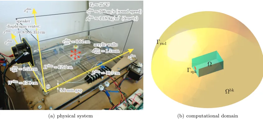
We consider the application of the PBDW framework to a physical system: a raised-box acoustic resonator. The system is depicted in Figure 2(a). We note that this problem was first considered in [16]; a detailed description of the physical system, data-acquisition procedure, and best-knowledge mathematical model is provided in [16]. We provide here only a brief overview of the raised-box acoustic resonator system and the experimental protocol. We instead focus on providing a more detailed analysis and interpretation of the data assimilation results.
5.2.
System Configuration
By way of preliminaries, we introduce a nondimensional frequency,
˜ k≡2π
˜ fdimr˜dimspk
˜ cdim
0
,
where ˜fdim is the driving frequency of the speaker, ˜rdim
spk ≈2.54cm is the radius of the speaker diaphragm, and ˜cdim0 ≈346m/s is the speed of sound. Here the tilde (˜·) implies that the quantity is ameasured quantity. Note that ˜k may also be interpreted as the measured nondimensional wavenumber.
We then define a system configuration
C= (˜k, box dimensions, box material properties, speaker placement,
speaker characteristics, temperature, extra-box environment, . . .).
(a) physical system (b) computational domain
Figure 2. The raised-box acoustic resonator and the robotic observation platform: (a) the
physical model, and (b) the best-knowledge computational domain. The figures reproduced with permission from [16].
We distinguish the nondimensional frequency ˜k— which we will actively vary and control — from all other properties that define the configuration and over which we have no control. To make the distinction more explicit, we denote the configuration of the acoustic resonator driven at the nondimensional frequency ˜kby
C˜k.
5.3.
Robotic Observation Platform
We perform autonomous, rapid, and accurate data acquisition using a robotic observation platform. A microphone mounted on a three-axis actuation platform measures the time-harmonic acoustic pressure of the system in the configurationC˜kat the specified location. We next convert the time-harmonic signal to complex pressure, ˜pdim
m , through a least-squares fit. The error in the time-harmonic complex pressure is estimated to be
about 5%. This error includes not only the noise-induced stochastic error considered in Section 3.3, but also the error associated with the calibration of the instruments. The error also includes the effect of inevitable variations in the configuration during the data-acquisition sequence; in actual physical experiments, unlike in the ideal abstract setting we have considered, we cannot perfectly maintain the configurationC˜kinvariant. We refer to [16] for detailed descriptions of the microphone calibration and validation procedures. We take these pressure observations as effectively “exact”; more precisely, we will only attempt to assess the accuracy of the data assimilation procedure to the 5% error level consistent with the observations.
We now normalize ˜pdimm [C˜k] as
˜ ym[C˜k] =
˜ pdim
m [Ck˜] ˜
ρdim 0 ˜cdim0 V
bk,dim spk (˜k)
, (17)
where, ˜ρdim
0 ≈1.18kg/m3is the density of air, andV
bk,dim
spk (˜k) is the speaker diaphragm velocity deduced from the speaker best-knowledge model introduced below. For the purpose of PBDW estimation and subsequent assessment, we collect 84 observations on a 7×4×3 axis-aligned grid for each nondimensional frequency ˜
k∈[0.3,0.7].
5.4.
Best-Knowledge Model and Imperfections
We now introduce our parametrized best-knowledge model. The model is defined over an extended domain Ωbk ⊂Ω shown in Figure 2(b), such that a radiation boundary condition can be specified away from the
acoustic resonator itself; the details of this “super-domain” formulation is provided in [16]. The model consists of two parameters: the nondimensional frequencyk∈ Dk ≡[0.3,0.7]; the speaker amplification and
phase-shift factorγ∈ Dγ ≡C. We now introduce the best-knowledge nondimensionalized pressure field,
ubk,µ≡ pbk,µ,dim
ρdim 0 cdim0 V
bk,dim spk (k)
, (18)
as the solution of the following weak statement: givenµ≡(k, γ)∈ Dk× Dγ ≡ D, findubk,µ∈ Ubk≡H1(Ωbk)
such that
a(ubk,µ, v;µ) =f(v;µ) ∀v∈ Ubk,
where
a(w, v;µ)≡ Z
Ω
∇w· ∇vdx¯ −k2
Z
Ω
wvdx¯ +
ik+ 1 R
Z
Γrad
w¯vds ∀w, v∈ Ubk,
f(v;µ)≡ikγ
Z
Γspk
1¯vds ∀v∈ Ubk.
We model the time-harmonic propagation of the sound wave in air by the Helmholtz equation. We model the walls of the raised-box resonator by a homogeneous Neumann boundary condition, which imposes infinite acoustic impedance. We model the time-harmonic forcing generated by the speaker as a uniform Neumann condition over Γspkof magnitudek→γVbk,dim(k), whereVbk,dim(k) is derived from a second-order oscillator model for the electromechanical speaker; note this model appears in our equations indirectly through the nondimensionalization of (18) and directly in the Neumann condition on Γspk through the γ (amplitude) and “1” (spatial uniformity). We model the radiation into free space by a first-order radiation condition on Γrad; the radiation term also ensures that the problem is well-posed for all µ∈ D. We approximate the solution by a finite element solution associated with a 35,325-elementP3 space.
While we choose the best-knowledge model to reflect our best-knowledge of the physical problem (subject to experimental and computational constraints), the model is not perfect. Here we identify some anticipated model imperfections and hence unmodeled physics.
The first set of imperfections is associated with our speaker model, k → γVbk,dim(k). First, the real speaker may exhibit non-rigid diaphragm motion, which is not captured by our uniform-velocity speaker model. Second, the real speaker may exhibit nonlinear response, which is not captured by our second-order harmonic oscillator model. Third, the real speaker may experience feedback from the variation in the pressure inside the box, which is not captured by our Neumann speaker model. Fourth, the real speaker may not be mounted perfectly symmetrically about the x2 plane, unlike the perfectly centered Γspk of our mathematical model. As we will see shortly, this unmodeled asymmetry in the speaker can have a significant consequence: on one hand, every solution to our mathematical model is symmetric about thex2 plane, and hence our background space is symmetric about thex2 plane; on the other hand, the slightest asymmetry in the speaker location can excite non-symmetric modes, especially when the speaker is operating near an anti-symmetric resonance frequency.
The second set of imperfections is associated with our wall model. First, the real wall is elastic and has a finite and spatially varying acoustic impedance, which is not captured by the perfectly rigid (infinite impedance) wall of our best-knowledge model. Second, the real elastic wall provides a dissipative mechanism through damping which is again not captured by the rigid wall of our best-knowledge model. Third, the real raised-box enclosure has fasteners and joints not captured by the homogeneous wall of our best-knowledge model.
The third set of imperfections is associated with our radiation model. The real acoustic resonator is not placed in a free space, and the pressure field inside the box can be affected by various environmental factors. We now turn to the prior prediction and prior prediction error. For the prior prediction, we take the best-knowledge solution ubk,µ at µ = µbk = (kbk = ˜k, γbk = 1). The prior prediction shall perforce suffer
N
0 2 4 6 8 10
0
b
k
;
D
d
is
c
;N
es
ti
m
a
te
10-2 10-1 100
Figure 3. Convergence of the discretization error.
incurred due to the choice ofµbk. (It is less that the prior prediction suffers from an incorrect choice of these
parameters, and more that the best-fit-over-manifold can exploit flexibility in these parameters within the Helmholtz structure. In particular, the best-fit-over-manifold can benefit from a choice ofk different from kbk= ˜k(even though ˜kis an accurate measurement of the actual frequency) and a choice ofγdifferent from
γbk= 1 as a way to represent a shift in resonance frequency and modification of amplitude and phase due
in fact to the imperfect modeling of wall interactions, damping, and speaker.)
5.5.
PBDW Formulation
We first introduce Hilbert spaceU ≡H1(Ω) endowed with a weightedH1 inner product
(w, v)≡ Z
Ω
∇w· ∇vdx¯ +k2ref
Z
Ω
wvdx¯ ∀w, v∈ U,
and the associated induced normkwk ≡p
(w, w); we choose kref = 0.5 as the reference frequency.
We next introduce the background space. The background space is generated in two steps: we first apply the WeakGreedy algorithm to Mbk ≡ {ubk,µ | µ ∈ D} to obtain hierarchical reduced basis spaces Zbk
N ≡span{ubk ,µˆn}N
n=1,N = 1, . . . ,8≡Nmax; we then restrict the functions over Ωbkin ZNbk to the domain
of interest Ω to formZN ≡ {z∈ U |z=zbk|Ω, zbk∈ ZNbk},N = 1, . . . , Nmax. Note that this procedure, which first computes the basis over Ωbk and then restricts the basis to Ω⊂Ωbk, can generate an ill-conditioned
basis if any two basis functions differ only over Ωbk\Ω; a more stable approach is to work on functions
restricted to Ω⊂Ωbk in the initial selection of the basis functions. However, this latter procedure requires
non-trivial localization of residual and does not permit the direct application of theWeakGreedy algorithm, which operates on the PDE defined over Ωbk. Note also that if the localized basis is ill-conditioned, then we
could apply POD and discard unnecessary elements to improve the conditioning. In any event, we do not encounter this ill-conditioning issue in our raised-box acoustic resonator.
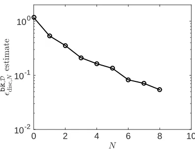
We show in Figure 3 the convergence of an estimate of the discretization errorbkdisc,D,N ≡supw∈Mbkinfz∈ZNkw−
zk; recall that (RZN1), in view of (16), requires a small discretization error. Thanks to the judicious choice
of the snapshots by theWeakGreedyalgorithm, the discretization error decays rapidly withN.
We next introduce the observation functionals and the associated experimentally observable update space. We model the experimental observations provided by the microphone with Gaussians,`om≡Gauss(·;xcm, rm=
0.2). We then form a libraryL of 84 observation functionals consistent with the dataset described in Sec-tion 5.3. We apply the SGreedyalgorithm to the libraryL andZNmax to choose a sequence of observation
functionals, `o
m, m = 1, . . . ,48 ≡Mmax, that maximizes the stability constant βN,M. We finally form the
associated experimentally observable update spaces,UM ≡ {qm≡RU`mo}Mm=1,M = 1, . . . , Mmax. Note that the precise choice of the filter widthrmis not important here since the microphone dimension is quite small
compared to the wavelengths of interest.
M
100 101 102
-N
;M
10-1 100
N= 2
N= 5
N= 8
(a) inf-sup constant
M
100 101 102
tr
a
ce
(
A
!
1)
100 101 102 103
(b) observation-conditioning metric
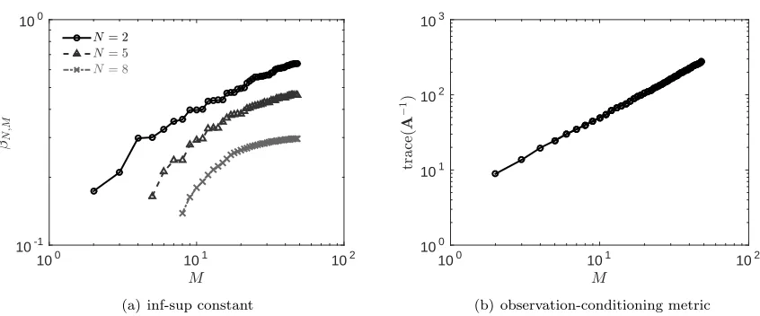
Figure 4. Behavior of the stability constantβN,M and the observation-conditioning metric trace(A−1).
We show in Figure 4(a) the behavior of the stability constantβN,M; recall that (RUM1) requires the
inf-sup constant to be away from zero and close to the unity. We note that the inf-inf-sup constant associated with the observation sequence identified by SGreedyis considerably larger than the inf-sup constant associated with a random sequence of observations, as demonstrated in [16]. The SGreedy algorithm ensures that this requirement is satisfied. We show in Figure 4(b) the behavior of the observation-conditioning metric trace(A−1); recall that (R
UM3) requires that trace(A
−1) is not too large. Because the transducers have relatively narrow filter width, and the maximization of the stability constant bySGreedytends to result in the selection of observation centers that are distant from each other, the observations are well-conditioned; in particular, we do not observe the exponential divergence observed for some cases in Figure 1. In conjunction with the relatively small observation error of 5% as reported in Section 5.3, we conclude that the stochastic error is relatively small, and in any event does not grow exponentially withM.
5.6.
Real-Time
In Situ
State Estimation
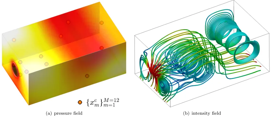
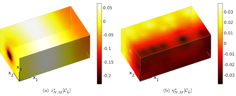
We now report a typical data assimilation result. Figure 5(a) shows the imaginary component of the time-harmonic pressure field for ˜k= 0.69 estimated from the PBDW formulation for a N = 7 dimensional background space and M = 12 observations. The observation points are depicted by the orange dots. Although the 12 observations arguably provide only sparse coverage relative to the complexity of the field, we are able to recover a qualitatively convincing pressure field thanks to the information provided by the background space. (We will quantitatively confirm in Section 5.7 that the estimated field is indeed a good approximation of the true pressure field.)
The PBDW formulation provides a full state estimation, and hence we may compute other derived fields of engineering interest, such as the sound intensity field depicted in Figure 5(b). For a time harmonic field, the sound intensity is related to the pressure field by
Iavg=<
−i 4πρ˜dim
0 f˜dim
pdimN,M∇p¯
dim
N,M !
,
where<(·) takes the real component of the complex number, andpdim
N,M is the dimensional pressure. We may
readily post-process the pressure field to obtain the sound intensity field. We observe in Figure 5(b) that the sound intensity is highest near the speaker. We note that the sound intensity exhibits a rather complicated structure even for this relatively simple acoustics problem.
We make a few remarks about the timing associated with data acquisition, data assimilation, and render-ing. The robotic observation platform requires on average little over 3 seconds per observation to reposition the microphone and to acquire the time harmonic signal. The acquisition of theM = 12 observations hence
(a) pressure field (b) intensity field
Figure 5. TheN = 7,M = 12 PBDW estimate of the (a) pressure field and (b) intensity
field for the normalized frequency of ˜k= 0.69.
takes approximately 40 seconds. The solution of the saddle system of size N+M = 19 takes less than 0.1 milliseconds on a laptop. The rendering of the solution using the current implementation takes approxi-mately 0.8 seconds; we speculate that this time can be significantly reduced by optimizing the rendering procedure at the software and hardware level. In any event, the total online time is dictated by the data acquisition step and is approximately 3M seconds.
5.7.
Error Analysis and Interpretations
5.7.1. Assessment Procedure
From the 84 observations we collect, we chooseJ = 36 observations associated with observation functional centers{ξc
m}Jj=1=36 as assessment observations. We ensure that the observation centers{xcm}
Mmax=48
m=1 used in the PBDW state estimation and the observation centers {ξc
m}Jj=1=36 used in the assessment are mutually exclusive: ξc
j ∈ {/ xcm} Mmax
m=1,j = 1, . . . , J. We then introduce the following pressure estimates associated with the assessment observations:
Pprior(j; ˜k)≡Gauss(ubk,µbk=(kbk≡˜k,γbk≡1)
;ξjc,0.2),
PN,M∗ (j; ˜k)≡Gauss(u∗N,M[Ck˜];ξjc,0.2),
Ptrue(j; ˜k) = (nondimensionalized experimental observation (17)
atξcj for configuration C˜k),
where Ck˜ specifies the experimental configuration. Throughout the assessment process, we take the assess-ment observation as the “truth”; more precisely, as noted in Section 5.3, we will only attempt to assess the state error to the observation error level,≈5%, such that the observations can serve as a surrogate for the truth. We finally introduce ana posteriori error indicator,
Eavg[C˜k]≡
v u u t
1 J
J X
j=1
|Ptrue(j; ˜k)−P∗
N,M(j; ˜k)|2; (19)
~ k
0.3 0.4 0.5 0.6 0.7
am
p
li
tu
d
e
10-2 10-1 100 101
Pprior(j; ~k)
P$
N=7;M=12(j; ~k)
Ptrue(j; ~k)
~ k
0.3 0.4 0.5 0.6 0.7
p
h
as
e
-3.14 -1.57 0.00 1.57 3.14
Pprior(j; ~k)
P$
N=7;M=12(j; ~k)
Ptrue(j; ~k)
(a)ξc
j= (2.67,2.67,4.50)
~ k
0.3 0.4 0.5 0.6 0.7
am
p
li
tu
d
e
10-2 10-1 100 101
Pprior(j; ~k)
P$
N=7;M=12(j; ~k)
Ptrue(j; ~k)
~ k
0.3 0.4 0.5 0.6 0.7
p
h
as
e
-3.14 -1.57 0.00 1.57 3.14
Pprior(j; ~k)
P$
N=7;M=12(j; ~k)
Ptrue(j; ~k)
(b)ξc
j= (9.33,2.67,4.50)
Figure 6. Frequency response (amplitude and phase) at the assessment center (a) ξcj =
(2.67,2.67,4,50) and (b)ξc
j = (9.33,2.67,4.50).
here, we recall thatN is the dimension of the background space,M is the dimension of the observable space, J is the number of assessment observations, and ˜k is the operating frequency. A formulation and analysis for this experimentala posteriori error estimate is provided in [19].
5.7.2. Frequency Response
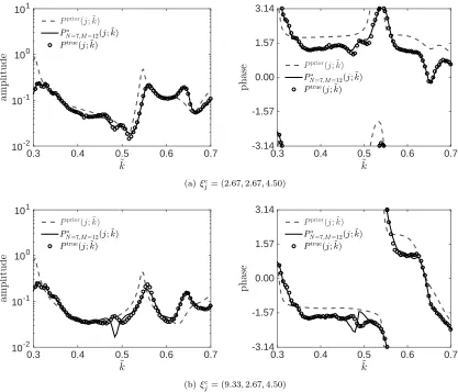
We first study the frequency response obtained at a single observation point. In Figure 6(a), we compare three frequency response curves observed atξc
j = (2.67,2.67,4.50): the prior prediction; the prediction by the
N = 7,M = 12 PBDW estimate; and the value observed by the microphone, which we take as the truth. We observe that the prior prediction differs considerably from the truth. The prior prediction overestimates the amplitude near the resonances and underestimates the resonance frequencies; we speculate the discrepancy arises from the use of the perfectly rigid wall in the best-knowledge model. The model also suffers from a phase shift. The PBDW estimate closely tracks the truth frequency response over the entire frequency range, in part due to the parametric flexibility provided in the speaker model, γ6=γbk = 1, in part due to
the intrinsic flexibility of model superposition provided by our linear space. (In actual practice, the former and latter are not distinguishable.)
We compare in Figure 6(b) the frequency response curves observed at ξjc = (9.33,2.67,4.50). We again observe that the prior prediction overestimates the resonance amplitude, underestimates resonance frequency,
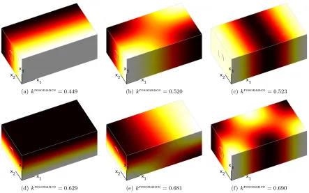
(a)kresonance= 0.449 (b)kresonance= 0.520 (c)kresonance= 0.523
(d)kresonance= 0.629 (e)kresonance= 0.681 (f)kresonance= 0.690
Figure 7. Resonance modes associated with the simple Neumann box.
and leads in the phase. The PBDW estimate again closely tracks the truth frequency response over the entire frequency range, except at near ˜k= 0.48.
We may explain the discrepancy observed near ˜k = 0.48 through the resonance modes associated with the acoustic resonator. To simplify the analysis, we consider here a simple box-only configuration with homogeneous Neumann boundary condition on all six sides of the box. The resonance modes in the frequency rangeDk˜≡[0.3,0.7] are shown in Figure 7. The inaccuracy of the PBDW estimate for ˜k≈0.48 is due to the
x2-antisymmetric resonance mode shown in Figure 7(a). The physical system is inevitably asymmetric about thex2-plane; for instance, the speaker is not mounted in the box precisely symmetrically and furthermore does not vibrate precisely symmetrically. Hence, in the physical system,x2-antisymmetric resonance modes are excited. In contrast, the best-knowledge model, for allµ∈ D, is perfectly symmetric about thex2plane, and hence only the symmetric resonance modes are excited. Hence, we expect significant (relative) model error for frequencies ˜k that are close to antisymmetric resonances but are far from symmetric resonances: ˜
k= 0.48 satisfies this requirement.
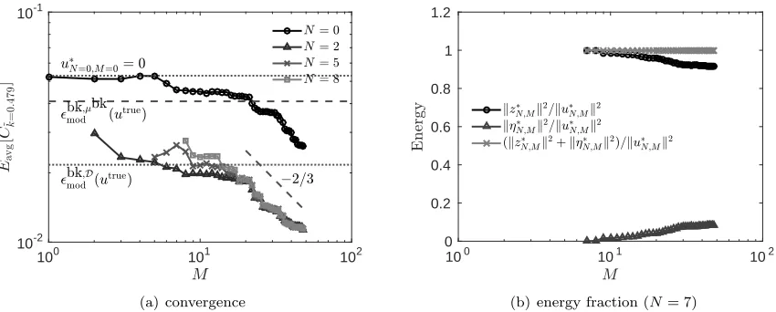
5.7.3. Convergence: x2-Symmetric Resonance
We now study the convergence behavior of the PBDW estimate for two different configurations: one near thex2-symmetric resonance at ˜k= 0.557 and the other near thex2-antisymmetric resonance at ˜k= 0.479. We first study thex2-symmetric resonance at ˜k = 0.557. For this configuration, the x2-asymmetry in the physical system is unimportant because ˜kis near the (shifted) symmetric resonance depicted in Figure 7(b). (The shift in the resonance frequency arises due to the difference in the wall boundary conditions: the wall of the mathematical model is perfectly rigid; the real wall is elastic.) We hence expectutrue[C˜k] to be close
to the best-knowledge manifoldMbk, and the model errorbk,D mod(u
true[C ˜
k]) to be small.
We show in Figure 8(a) the convergence of the PBDW estimate with the background space dimensionN and the number of observations M. We also show the errors associated with three different estimates: the error associated with the zero estimateu∗N=0,M=0 = 0 (note that this “error” is in fact just the magnitude
ofutrue[C˜k]); the error associated with the prior predictionubk ,µbk