A galerkin boundary element method for solving the generalized Helmholtz decomposition

A Galerkin Boundary Element Method for Solving

the Generalized Helmholtz Decomposition

*

S. N. Kempka ([email protected]) M. W. Glass ([email protected]) J. H. Strickland ([email protected])

Engineering Sciences Center Sandia National Laboratories Albuquerque, NM 87185, USA

M. S. Ingber

Department of Mechanical Engineering University of New Mexico Albuquerque, NM 87106, USA

Abstract

The objective of this work is to more accurately calculate velocities, particularly on boundaries, by using the Galerkin form of the generalized Helmholtz decomposition. This work describes advantag-es of using the generalized Helmholtz decomposition over other formulations and shows the accuracy and convergence advantages of Galerkin numerical methods over point collocation methods. Solu-tions based on Galerkin and point collocation methods are compared for two-dimensional problems. The comparison shows that Galerkin solutions are significantly more accurate and less oscillatory. Accordingly, the Galerkin method is recommended for use with vortex methods.

1. Introduction

Vorticity formulations of the incompressible Navier-Stokes equations require the determination of the ve-locity field from the vorticity field and the normal veve-locity boundary condition. An often-used formulation for the velocity is

, (1)

where is the velocity induced by the vorticity field in the infinite domain ,

, (2)

with

,

the gradient of the infinite domain Green’s function for Poisson equations, and d = 2 for two-dimensional flow, and d = 3 for three-dimensional flow. Variables of integration are denoted with primes. Eq. (2) is of-ten referred to as the Biot-Savart Law.

The last term, is a velocity field that is irrotational, as imposed by its form ( ), and is diver-gence free, as imposed by the governing equation for the velocity potential, ,

in the fluid domain (3)

The normal velocity boundary condition, , ( is the outward pointing unit normal vector) is imposed as a von Neumann boundary condition on Eq. (3) (assuming and are specified),

. (4)

u

˜ u

˜

u

˜ω

∇φ

+ =

u

˜ω

ω = ∇×u R_∞

u

˜ω

x

˜

( ) ω

˜

x' ( ) g

˜

x

˜

x

˜ '

,

( )

× R x

˜ '

( ) d

R_∞

∫

=

g

˜

x

˜

x'

˜

,

( ) 1

2π(d–1) ---(x_˜–x'_˜ )

x–x'd

---=

∇φ ∇ ∇φ× ≡0

φ

∇ ∇φ• = 0

nˆ•u nˆ

ω = ∇×u D = ∇•u nˆ•∇φ nˆ u

˜

u

˜ω –

[ ]

•

Eq. (4) shows how spatial variations in result in variations in the von Neumann boundary condition on Eq. (3). Note that the tangential velocity on the boundary is determined as part of the solution of Eq. (3),

i.e., the solution contains the tangential velocity .

The focus of this work has been to obtain accurate tangential velocities on the boundary. The tangential ve-locity is crucial to predicting flow stability and is the basis for vorticity creation in some formulations. Er-rors can arise from a variety of sources. Methods based on solving the differential equation Eq. (3) yield tangential velocity errors as a result of approximate derivatives on the boundary. Boundary element solu-tions to Eq. (3) have superior convergence properties but suffer from the same difficulties when applying gradient operators (discrete and analytical) to the potential function. Large errors in the tangential velocity on the boundary can also occur if spatial variations in the normal velocity boundary condition are not accu-rately resolved.

This paper presents the generalized Helmholtz decomposition (GHD) as an alternate formulation that avoids the errors in the tangential velocity by allowing boundary velocities to be calculated directly, i.e., without the use of an intermediate potential function. The GHD is solved using Galerkin and point colloca-tion methods. Galerkin methods more accurately resolve variacolloca-tions in the normal velocity boundary condi-tion and, therefore, are expected to yield more accurate solucondi-tions. Indeed, the Galerkin method is shown to be significantly more accurate and more convergent than point collocation methods. Analysis of the Galer-kin formulation also allows insight into the appropriate use of the GHD and provide the basis for estimat-ing the error in the solution before the solution is computed.

2. Governing Equations: The Generalized Helmholtz Decomposition

The specification of an incompressible velocity field, in terms of the vorticity field and the normal velocity boundary condition, is provided by the generalized Helmholtz decomposition

(5)

, where is the internal angle of the boundary. For points on smooth bound-aries . For two-dimensional flow d = 2, and for three-dimensional flow d = 3. The fluid do-main is denoted by R, and its surface is denoted by S. Primes indicate variables of integration. The unit normal vector is .

Equation (5) has been derived by numerous authors: see references from 1941 to 1996, Stratton [11], Mor-se and Feshback [10], Byhkovskiy and Smirnov [2], Wu et. al [14][15][16][17], Morino [8][9], Uhlman and Grant[13], Meir and Schmidt [7], Casciola et al [3].

Next we consider the determination of the tangential velocity from Eq. (5) (evaluated on the boundary), as-suming that the normal velocity boundary condition, , and vorticity are specified. For three-dimen-sional flows the unknown tangential velocity is contained in the vortex sheet, , which has three non-normal components (in general x, y, and z directions) so Eq. (5) has three components. Thus, there is an equation for each component of the unknown tangential velocity, allowing it to be readily determined. For two-dimensional flows the unknown tangential velocity is contained in the vortex sheet , whose direction is out of the plane, ), so the unknown has only one component. Eq. (5), however, has two components. Thus, in two-dimensional problems it must be determined which component of Eq. (5) should be solved.

u

˜ω

∇φ nˆ×∇φ×nˆ

x

˜

in R: u ˜ x ˜ ( ) x ˜

on S: α x

˜

( )u

˜ x ˜ ( ) x ˜

outside R: 0 ˜      ω ˜ x' ( ) g

˜ x ˜ x ˜ ' , ( )

× R x

˜ ' ( ) d R

∫

=

+ nˆ x

˜ '

( ) u

˜ × x ˜ ' ( ) –

[ ] g

˜ x ˜ x ˜ ' , ( )

× S x

˜ '

( ) d

S

∫

nˆ x

˜ '

( ) u

˜ • x ˜ ' ( ) [ ] –

( )g

˜ x ˜ x ˜ ' ,

( ) S x

˜ ' ( ) d S

∫

+

α( )x = Λ( )x ⁄2π(d–1) Λ( )x α( )x = 1 2⁄

nˆ

nˆ•u

nˆ×u

To examine this issue, we express the velocity on the left-hand side of Eq. (5) in terms of its nor-mal component and its tangential component, the latter of which can be expressed in terms of the unknown vortex sheet . Rearranging Eq. (5) (evaluated on the boundary) to isolate all terms containing the unknown vortex sheet strenght on the left-hand side, and denoting all other terms (which are known quantities) as on the right-hand side, we obtain as new representa-tion of Eq. (5)

. (6)

Eq. (6) is a vector Fredholm equation in which the normal and tangential components are both sat-isfied by the solution . The question addressed here is whether there is an advantage to solving the normal or tangential component.

The normal component of Eq. (6) is a Fredholm equation of the first kind for the unknown (since does not appear on the left-hand side of the normal component of Eq. (6)) thus any discrete for-mulation will yield a matrix that is not diagonally dominant.

The tangential component of Eq. (6) is a Fredholm equation of the second kind for the unknown , (since appears on the left hand side of the tangential componenet of Eq. (6)) thus any discrete formulation will yield a diagonally dominant matrix.

This analysis would seem to indicate that the tangential component is more suitable for numerical analysis. However, there are other issues to consider, such as how this behavior is reflected in the numerical method, and the existence of the solution for multi-ply connected domains, which will be described next. In particular, it will be shown that for the Galerkin method, the normal compo-nent yields a rank deficient matrix, and the tangential compocompo-nent requires the application of a con-straint to ensure existence of a solution.

3. Discretization of the Governing Equation

A weighted residual approach is discussed in which the governing equation ( ) is multi-plied by a weighting function, , and integrated over the boundary

. (7)

If the weighting function is a delta function , a point collocation method is ob-tained with collocation points at locations . With point collocation information is used only at discrete points. If on an element and 0 elsewhere, a Petrov-Galerkin method is ob-tained. Petrov-Galerkin methods yield a solution that satisfies the governing equation in an integral sense but not pointwise. An intermediate approach is a Galerkin method in which the weighting functions are the basis functions used to represent spatial variations over a finite element. Since the basis functions are a function of space, some point-wise information is included in addition to some integral information. This approach has been found to provide useful solutions for a wide va-riety of equations.

To obtain a discrete version of Eq. (7), the boundary is discretized into N_e boundary elements, with basis functions , that have N_b nodes on each element. A Galerkin form of Eq. (7) is obtained by using the basis function of each element as the weighting function and integrating over the en-tire boundary (where the basis functions are zero outside the element to which they belong). Let represent either the normal unit vector or the tangential unit vector . To further simplify the no-tation, the differential arc length, ds, is omitted from the line integrals. Either component is then represented as

γ

˜

x

˜

( ) nˆ x

˜

( ) ×

h x

˜

( )

γ

˜

x

˜

( ) g

˜

x

˜

x

˜ '

,

( )

× S x

˜ '

( )

d α x

˜

( ) γ

˜

x

˜

( ) nˆ x

˜

( ) ×

[ ]

+

S

∫

h x

˜

( )

=

γ

˜

nˆ

– u

˜

×

=

γ

˜

γ

˜

γ

˜

γ

˜

f x

˜

( ) = 0

w x( )

w x

˜

( )f x

˜

( )

S

∫

dS x

˜

( ) = 0

w x

˜

( ) δ x

˜

x

˜

e_i,n_j

–

( )

=

x

˜

ei,nj w x( ) = 1

Φe_i,n_j

υˆ

, (8) for 2D, where the coefficient is defined as

.

The quantity denotes the velocity induced on element k by the vortex sheet associated with the j-th basis function on element i. is the Kronecker delta function.

To obtain linear

coeffi-cients for the vortex sheet nodal values,

let

. The resulting

discretized governing equation is a set of linear equations described by

. (9)

Detailed consideration of any column in the matrix reveals that the sum of the matrix entries in any column is the numerical approximation to the boundary integral of the velocity (normal or tangential) induced by the single vortex sheet associated with that column, as indicated by

. (10)

The left-hand side of Eq. (10) is the sum of the marix entries in any column, and the right-hand side de-notes the analytical representation of the boundary integral of the velocity (either normal or tangential, as specified) induced by a vortex sheet defined by the nodal value and the j-th basis function, , on element e_i.

For normal and tangential components of velocity, the boundary integrals on the right-hand side of Eq. (10) are related kinematically to other known quantities. This observation can be used to indicate the accuracy of the numerical method used to evaluate the left-hand side of Eq. (10) and to show which component of the governing equation should be solved, as discussed below.

For the normal component ( ), Eq. (10) is the integral of the normal velocity induced by the vortex sheet over the boundary. This quantity is related to the divergence of the velocity by the diver-gence theorem

. (11)

For incompressible flows , so that from Eq. (11), .

Thus, if the normal component of the governing equation is used, the sum of all elements in a column should be zero for every column. In any column sum, the nodal value of the vortex sheet is constant. Thus, for the normal component of the governing equation and , the constant value can be eliminated from the column sum, with no loss of generality, to obtain the analytical result,

. (12)

υˆ_e

k Φek,nl γ

˜

e_i,n_j β

˜

e_i,n_j( )ek

×

j=1

N_B

∑

i=1

N_e

∑

e_k

∫

• υˆ_e

k Φek,nlh

˜

e_k

∫

•

=

υˆ _{= nˆ or τ}ˆ _β

e_i,n_j( )ek

β

˜

e_i,n_j( )ek δi k, δj l, αe_iΦe_i,n_jnˆe_i Φe_i,n_j g

˜

x

˜

e_i x

˜ e_k , ( ) e_i

∫

+ = γ ˜

e_i,n_j β

˜

e_i,n_j( )ek

×

δa b,

γ

˜

e_i,n_jηe_i,n_j( )ek υˆek γ

˜

e_i,n_j β

˜

e_i,n_j( )ek

×

[ ]

•

=

Φe_k,n_l γ

˜

e_i,n_jηe_i,n_j( )ek j=1

N_B

∑

i=1

N_e

∑

e_k

∫

υˆ_e

k Φek,nlh

˜

e_k

∫

•

=

Φe_k,n_lγ

˜

e_i,n_jηe_i,n_j( )ek e_k

∫

l=1

N_b

∑

k=1

N_e

∑

γ

˜

e_i,n_jηe_i,n_j

∫°

=

γe_i,n_j Φe_i,n_j

υˆ _{= nˆ}

γe_i,n_jΦe_i,n_j

nˆ u

˜

• ( )ds

∫°

∇ u

˜

• ( )dA

A

∫

=

∇•u = 0 nˆ u

˜

• ( )ds

∫°

= 0

γei,nj ∇ u

˜

• = 0 γe_i,n_j

ηe_i,n_j e_k

∫

k=1

N_e

In this case where every column sum is zero analytically, then any particular row equals the oppo-site of the sum of all the other rows. As a result, an entire of row of zeros can be obtained, indicat-ing that the matrix is rank deficient. Thus, this analysis shows (analytically) that the normal component of the governing equation yields a rank deficient matrix. This indicates that the normal component of the governing equation should not be used.

For the tangential component of the governing equation, , the column sum, Eq. (10), is the integral of the tangential velocity over the entire boundary. Stokes’ theorem (or the theorem of the rotational) states that this boundary integral of the tangential velocity is equal to the domain inte-gral of the vorticity

. (13)

(A three-dimensional version of this identity also exists.) Recall that the sum of the entries in a col-umn of the matrix corresponds to the boundary integral of the tangential velocity induced by the vortex sheet specified by the nodal value and the j-th basis function on element e_i, . This quantity corresponds to the left-hand side of Stokes’ theorem.

(14) For a 2-D interior flow, the right-hand side of Stokes’ theorem is evaluated by considering that the only vorticity in the problem is the vortex sheet . The area integral of the vorticity for this special case is

(15) Thus, for a 2-D interior flow, if the tangential component of the governing equation is used, Stokes’ theorem indicates that the sum of each column should be, eliminating the vortex sheet nod-al vnod-alue , as before):

(simply connected domains). (16) This equation shows that the column sum is non-zero, and thus the matrix is not rank-deficient, suggesting that the tangential component is the appropriate component to be used for numerical computation.

The preceding discussion is appropriate for internal flows. In external flows there are well-known, additional features that must be considered. For example, consider flow around a cylinder in an in-finite domain. First, note that all vortex sheets associated with the tangential velocity on the bound-ary are outside the boundbound-ary of the cylinder so that the boundbound-ary does not enclose the vortex sheet. By Stokes’ theorem the integral over the entire cylinder boundary of the tangential velocity in-duced by any particular vortex sheet must be zero,

(multiply-connected domains). (17)

υˆ _{= τ}ˆ

u

˜

ds

˜

•

∫°

ω

˜

A

˜

d •

A

∫

=

γe_i,n_j Φe_i,n_j

u

˜

ds

˜

•

∫°

γ

˜

e_i,n_jηe_i,n_j e_k

∫

k=1

N_e

∑

=

γe_i,n_jΦe_i,n_j

ω

˜

A

˜

d •

A

∫

γ

˜

e_i,n_jΦe_i,n_jds e_i

∫

=

γe_i,n_j

ηe_i,n_j e_k

∫

k=0

Ne

∑

Φe_i,n_jds e_i

∫

=

γ

˜

e_i,n_jηe_i,n_j e_k

∫

k=0

Ne

This result shows that for an exterior flow, application of the Galerkin method to the tangential component of the governing equation yields a matrix in which the sum of each column is zero. As discussed for the case of the normal component of the governing equation, if each column sums to zero, the matrix is rank deficient. This rank deficiency is well-known for exterior problems. Methods to treat this problem are dis-cussed by Greenbaum, Greengard, and McFadden [4]. The fact that the Galerkin numerical formulation re-flects analytic rank deficiency is viewed as an advantage of the numerical method.

To summarize, a Galerkin formulation was presented for use in solving for the tangential velocity on the boundary given the normal velocity boundary condition and the vorticity field. Analysis of the formulation shows that the tangential component of the formulation should be used, since the normal component leads to a rank deficient set of equations. Next, numerical examples are presented to show the advantages of the Galerkin approach over the often-used point collocation method.

4. Numerical Examples

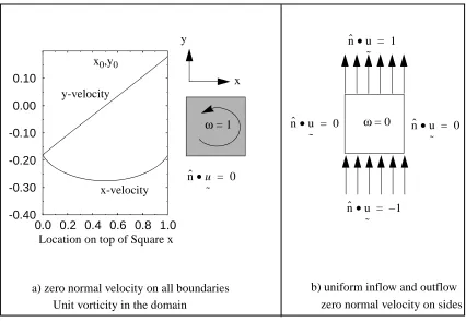
The Galerkin formulation and a point collocation formulation are applied to two flows in a two-dimension-al square domain shown in Figure 1. Linear boundary elements are used in each problem. The velocity in-duced by a linear vortex sheet on each boundary is known analytically [1].

The first problem has zero vorticity and uniform boundary conditions on each side (uniform inlet and out-let velocities on two opposing sides with zero normal velocity on the remaining sides). See Figure 1b. The

ω = 1 y

x

x-velocity y-velocity

0.0 0.2 0.4 0.6 0.8 1.0 -0.40

-0.30 -0.20 -0.10 0.00 0.10

Location on top of Square x x₀,y₀

Figure 1 Two flows used to compare the accuracy of Galerkin and point collocation solution methods. a) The unit square contains unit vorticity with zero normal velocity on all boundaries. The x and y velocity components induced on the top of the unit square by unit vorticity filling the square are shown. b) The unit square contains zero vorticity in the domain with uniform inlet and outlet velocities and zero normal velocity on the remaining sides.

a) zero normal velocity on all boundaries nˆ u

˜

• = 0

Unit vorticity in the domain

b) uniform inflow and outflow zero normal velocity on sides

ω = 0 nˆ u

˜

• = 0 _{nˆ u}

˜

• = 0

nˆ u ˜

• = –1 nˆ u

˜

analytical solution is a uniform flow: The tangential velocity on the inlet and outlet boundaries is zero, and the tangential velocity on the remaining sides is the same as the inlet and outlet velocity. For this simple problem highly accurate solutions (within 10-16 for double-precision calculations) are obtained for both Galerkin and point collocation methods for all discretizations. This excep-tional behavior occurs because the simple boundary conditions are resolved very well in each case. For the more difficult problem discussed next, the boundary conditions have non-trivial spatial variations that are resolved to differing extents by each method. As a result, the solutions are very different.

The second, more difficult problem has uniform vorticity in the domain and requires zero normal velocity on all boundaries, as shown in Figure 1a. Linear boundary elements were used with both Galerkin and point collocation methods, and discretizations of 10, 20, 100, and 200 elements per side are considered. For the point collocation method, the evaluation points were at the mid-point of each element.

The velocity induced by a uniform, square vorticity field is known analytically. The x and y veloc-ities on the boundary of the unit square are shown in Figure 1. This is a severe test of the method from the point of view that the normal velocity induced by the vorticity field at the corners changes sign from one side of the corner to the other.

Solutions for the tangential velocity were computed using linear boundary elements. Solutions will be shown for point collocation and Galerkin methods. A four-point Gaussian quadrature was used to evaluate the boundary integrals associated with the Galerkin method. For the point collocation solutions, the collocation point was the mid-point of each element. For simplicity all nodes shared by two elements were assumed to have the same value of , even at corners, which is valid for this problem but not in general.

5. Discussion of Results

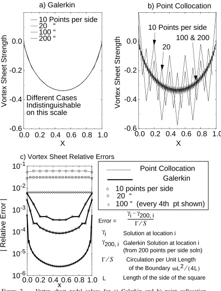
Figure 2 a and b shows the nodal values for several discretizations. The results show that the point collocation point solution oscillates for each of the discretizations, though the magnitude of the os-cillations decreases as the number of elements increases. The osos-cillations are visible, however, even with 200 boundary elements on one side of the square. The Galerkin solution does not show such oscillations for any of the discretizations.

Having shown the superior convergence properties of the Galerkin boundary element formulation, we now examine the accuracy of the solutions. This is important from the point of view that for constant density, incompressible flows, vorticity generation is often derived from the vortex sheets on the boundary. Thus, we wish to accurately calculate the vortex sheets.

Figure 2c shows an estimate of the relative errors based on the Galerkin solution for 200 points on a side. For any discretization the Galerkin solution is approximately ten times more accurate than the point collocation solution. In fact, relative errors show that the Galerkin solution with 10 points per side is more accurate everywhere than the point collocation solution with 100 points per side. The largest errors occur in the corners. This is due to the highly nonlinear velocity induced by one element in a corner on the other element in the corner, which is not adequately represented by the quadrature.

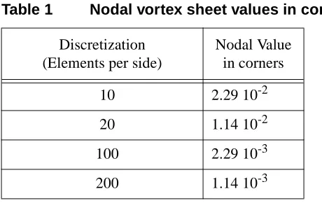
The analytic value of the vortex sheet strength in the corners is known to be zero. This result is de-termined from the (zero) normal velocities on the two elements comprising the corner and by re-quiring the x and y velocity components to be continuous in the corners, regardless of the direction from which the corner is addressed. Table 1 shows the nodal values in the corners. The non-zero values of the nodal values represent the absolute errors in the corners, and are seen to be

propor-γ

0.0 0.2 0.4 0.6 0.8 1.0

x

10

-6

10

-5

10

-4

10

-3

10

-2

10

-1

|

Re

la

tiv

e Err

o

r |

c) Vortex Sheet Relative Errors

0.0 0.2 0.4 0.6 0.8 1.0

-0.6

-0.4

-0.2

0.0

10 Points per side

20 “

100 “

200 “

0.0 0.2 0.4 0.6 0.8 1.0

-0.6

-0.4

-0.2

0.0

a) Galerkin

_{b) Point Collocation}

Vo

rt

e

x

Sh

ee

t

S

tre

ng

th

Vo

rt

e

x

Sh

ee

t

S

tre

ng

th

X

X

Point Collocation

Galerkin

10 points per side

20 “

100 “ (every 4th pt shown)

Error =

γ

_i

–

γ

_{200 i}

_,

Γ

⁄

S

---γ

_i

γ

_{200 i}

_,

Γ

⁄

S

Solution at location i

Galerkin Solution at location i

(from 200 points per side soln)

Circulation per Unit Length

ω

L2

⁄

(

4L

)

10 Points per side

20

100 & 200

Different Cases

Indistinguishable

on this scale

of the Boundary

L

Length of the side of the square

tional to the element size. (The large errors and low-order of the solution is being addressed using adaptive quadrature methods, such as described in Telles [12].)

6. Summary

The generalized Helmholtz decomposition was described for use as a formulation to enforce the normal velocity boundary condition when an incompressible velocity field is to be calculated from the vorticity field. The tangential velocity boundary condition is calculated directly in the general-ized Helmholtz decomposition, without the artifice of a velocity potential and its attendant difficul-ties.

In the two-dimensional problems considered, the vortex sheet has a single component (out of the plane), so a single component of the generalized Helmholtz decomposition (a vector equation) must be chosen. To address this issue, an analysis of the Galerkin formulation of the decomposi-tion was presented. The analysis showed that when considering the normal component of the de-composition, the column sum is always zero, which indicates that matrix is rank deficient and, therefore, is not a good choice for numerical solutions. On the other hand, a column sum for the tangential component of interior problems is equal to the non-zero integral of the vortex sheet as-sociated with that column. thus, the tangential component is the best choice of equations to solve for the unknown vortex sheet strength.

A comparison was made of solutions based on Galerkin and point collocation numerical methods. The Galerkin method was an order of magnitude more accurate and less oscillatory than point col-location methods for the general case where the normal velocity boundary condition has non-trivi-al spatinon-trivi-al variations. Point collocation methods simply do not represent these variations as well as the integral-based Galerkin method.

Future work is planned to explore the use of column sums as error indicators. In particular the col-umn sums are known so that the difference between the computed colcol-umn sum and the analytical value allow an assessment of the errors inherent in the numerical method. This observation might provide for the prediction of errors before the solution is obtained. Additional work is also planned to address the large errors that occur in corners. This will be critical in three-dimensional methods, where analytical solutions are not available for bilinear and higher-order elements, as they are in two-dimensions. As a result, quadratures will be needed for the integrals in the original general-ized Helmholtz decomposition, and the quadrature solutions are expected to introduce additional errors. Adaptive quadrature methods are anticipated to be useful to address this issue.

Table 1 Nodal vortex sheet values in corners.

Discretization (Elements per side)

7. References

1. J. H. Strickland, "A Vortex Panel Analysis of Circular Arc Bluff bodies in Unsteady Flow," AIAA 10-th Aerodynamic Decelerator Systems Technology Conference, April 18-20, 1989, Cocoa Beach, Florida

2. Byhkovskiy, E. B. and N. V. Smirnov, "On Orthogonal Expansions of the Space of Vector Functions which are Square-Summable over a Given Domain and the Vector Analysis Opera-tors," NASA TM-77051, 1983.

3. Casciola, C. M., Piva, R., and P. Bassanini, "Vorticity Generation on a Flat Surface in 3D Flows," J. Comp. Phys., vol. 129, pp. 345-356, 1996.

4. Greenbaum, A., Greengard, L., and G. B. McFadden, "LaPlaces’ Equation and the Dirichlet-Neumann Map in Multiply Connected Domains," J. Comp. Phys., vol. 105, pp. 267-278, 1993.

5. Kempka, S. N., M.W. Glass, J. H. Strickland, and M. S. Ingber, "Accuracy Considerations for Implementing Velocity Boundary Conditions in Vorticity Formulations," Sandia National Lab-oratories Report SAND96-0583, March 1996.

6. Lamb, H., Hydrodynamics, Sixth Edition, Dover Press, 1945.

7. Meir, A. J. and P. G. Schmidt, "Variational Methods for Stationary MHD Flow Under Natural Interface Conditions," J. Non-Linear Analysis-Theory, Methods and Applications, vol. 26, no. 4, p. 659-689, 1996.

8. Morino, L., "Helmholtz Decomposition Revisited: Vorticity Generation and Trailing Edge Condition," Computational Mechanics, vol. 1, pp. 65-90, 1986.

9. Morino, L., "Boundary Integral Equations in Aerodynamics," Applied Mechanics Reviews, vol. 46, no. 8, pp. 445,-466, August 1993.

10. Morse, P.M. and H. Feshback, Methods of Theoretical Physics, Part II, McGraw-Hill Publ. Co., 1953.

11. Stratton, J. A., Electromagnetic Theory, McGraw-Hill Book Company, 1941, p. 254.

12. Telles, J.C.F. and R.F Oliveira, "Third Degree Polynomial Transformation for Boundary Ele-ment Integrals: Further ImproveEle-ments," Engineering Analysis with Boundary EleEle-ments, vol. 13, pp. 135-141, 1994.

13. Uhlman and Grant, "A New Method for the Implementation of Boundary Conditions in the Discrete Vortex Element Method," ASME 1993 Fluids Engrg. Sprg. Mtg., Wash., D.C., June 1993.

14. Wu, J. C. and J. F. Thompson, "Numerical Solutions of Time-Dependent Incompressible Navi-er-Stokes Equations Using an Integro-Differential Formulation," Computers and Fluids, vol. 1, pp. 197-215, 1973.

15. Wu, J. C., "Numerical Boundary Conditions for Viscous Flow Problems," AIAA Journal, vol. 14, pp. 1042-1047, 1976.

16. Wu, J. C. and U. Gulcat, "Separate Treatment of Attached and Detached Flow Regions in Gen-eral Viscous Flows," AIAA Journal, vol. 19, no. 1, pp. 20-27, 1981.