Please cite this article as: E. Ahmadi, M. H. Abooie, M. Jasemi, Y. Zare Mehrjardi, A Nonlinear Autoregressive Model with Exogenous Variables Neural Network for Stock Market Timing: The Candlestick Technical Analysis, International Journal of Engineering (IJE), TRANSACTIONSC: Aspetcs Vol. 29, No. 12, (December 2016) 1717-1725
International Journal of Engineering
J o u r n a l H o m e p a g e : w w w . i j e . i rA Nonlinear Autoregressive Model with Exogenous Variables Neural Network for
Stock Market Timing: The Candlestick Technical Analysis
E. Ahmadi*a, M. H. Abooiea, M. Jasemib, Y. Zare Mehrjardia
a Department of Industrial Engineering, Yazd University, Yazd, Iran
bDepartment of Industrial Engineering, Khajeh Nasir Toosi University of Technology, Tehran, Iran
P A P E R I N F O
Paper history:
Received 19 February 2015
Received in revised form 09 September 2016 Accepted 08 October 2016
Keywords: Finance
Stock Market Forecasting Technical Analysis
NARX Recurrent Neural Network Levenberg–marquardt Algorithm
A B S T R A C T
In this paper, the nonlinear autoregressive model with exogenous variables as a new neural network is used for timing of the stock markets on the basis of the technical analysis of Japanese Candlestick. In this model, the “nonlinear autoregressive model with exogenous variables” is an analyzer. For a more reliable comparison, here (like the literature) two approaches of Raw-based and Signal-based are devised to generate the input data of the model. The correct predictions percentages for periods of 1- 6 days with the total number of buy and sell signals are considered. The result proves that to some extent the approaches have similar performances while apparently, they are superior to a feed-forward static neural network. The created network is evaluated by the measure of Mean of Squared Error and the proposed model accuracy is calculated to be extremely high.
doi: 10.5829/idosi.ije.2016.29.12c.10
1. INTRODUCTION1
Developing a model for predicting returns in order to make investment decisions is an important goal for academics and practitioners. Typically, the financial services industry relies on three main approaches to make investment decisions: 1- The fundamental approach that uses fundamental economic principles like economic, industry, and company conditions to form portfolios; 2- The Technical Analysis (TA) approach; and 3- The mathematical approach that is based on the mathematical model. The first two approaches dominate practice because of their applicability [1] and our paper focuses on the TA.
TA, also known as Charting has been a part of financial practice for many years. TA studies the historical data surrounding price and the volume movements of the stock by charts as the primary tool to forecast future price movements [2].
1*Corresponding Author‟s Email: [email protected] (E.
Ahmadi)
In recent years, TA has proven to be powerful for evaluating stock prices and is widely accepted among financial economists and brokerage firms. This is due to the fact that it offers a relative mixture of human, political, and economic events [2].
Xie et al. [6], Lan et al. [7], Chen et al. [8]. It is now accepted that stock markets are nonlinear dynamic systems; so linear approaches cannot identify the relationships in the time series of stock prices. However, an appropriate nonlinear model such as an intelligent system technique may be able to discover complex nonlinear relationships and handle the uncertainty and imprecision common in the stock market [2]. Artificial neural network (ANN), as the main approach in the field of Artificial Intelligence (AI), has attracted much interest over the past decade for its ability to forecast financial performance [8].
In this study, ANN is used as a computational intelligence because it typically performs well for classification, recognition, and forecasting of financial data and is capable of dealing with uncertain, fuzzy, or insufficient data that fluctuate rapidly in very short periods of time [2]. Many types of research have used ANNs in modeling and prediction of time series data [9-17]. Most of the reported research has focused on using feed forward neural network [18]. These networks do not have any feedback connections in their architectures. Therefore, they do not take into account the temporal dependencies between the data. Recurrent neural networks (RNNs) are widely used to deal with many dynamical and non-linear problems, including
time series prediction [19-21]. RNNs are
computationally more powerful than feed-forward networks and valuable approximation result has been obtained for prediction problems [18]. One of the most convenient forms among RNNs for prediction purposes is a nonlinear autoregressive model with exogenous variables (NARX) which is a quite general formulation where the current output value is made dependent on the past values of the input and output signals through a suitable nonlinear static function [20]. This type of ANN has been used in the work of Mahmoud et al. [18], Huo and Poo [22], Pisoni et al. [20], Andalib and Atry [19] as the prediction model, Sahooa et al. [23] for determination of the nonlinear systems, and Ardalani-Farsa and Zolfaghari [24] for the prediction and analysis of the chaotic time series. In this study, the key point about the model is the application of Japanese Candlestick technique.
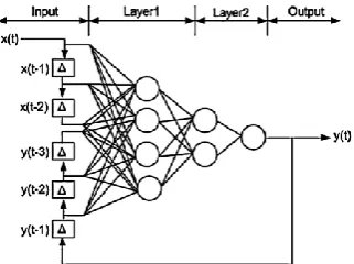
Figure 1. NARX network with two input delays and three
output delays
This study uses the NARX neural network in the field of Candlestick TA and compares the outputs with a feed-forward neural network.
The rest of the paper is organized as follows: section 2 reviews the literature of RNNs, NARX, and optimal architecture of an ANN; section 3 introduces the prediction model; section 4 presents the experimental results and finally section 5 focuses on the conclusions.
2. MATHEMATICAL MODEL
2. 1. RNN Generally, neural networks are two kinds of static and dynamic. Static networks have no feedback elements and no delays; the output is calculated directly from the current inputs and they assume that the data is concurrent and no sense of time can be encoded. These networks can thus lead to instantaneous21.
Dynamic networks may be difficult to train but are more powerful than static networks. As they have memory in form of delays or recurrent loops, they can be trained to learn sequential or time varying patterns. This makes them networks of choice for various applications like financial predictions, channel equalization, sorting, speech recognition, fault detection etc. Since we are dealing with a time series it is necessary to use dynamic networks. Dynamic networks are of two types: the ones with feed forward connections and taps; and those with feedback or recurrent networks [25].
2. 2. The NARX Network NARX is an important
class of discrete-time nonlinear systems. Not only are NARX neural networks computationally powerful in theory, but they have several advantages in practice. For example, it has been reported that gradient-descent learning can be more effective in NARX networks than in other recurrent architectures with „„hidden states‟‟ [22]. The key advantages of NARX network over other recurrent neural networks are its generalization and convergence at learning long-term dependencies. By long term dependencies, we mean the ability of the network to remember information that is stored for a long period of time [18].
Figure 1 shows the typical architecture of NARX network. In this model, Multi-Layer Perceptron (MLP) is used to approximate the following function.
)) ( ),..., 2 ( )), 1 ( ), ( ),..., 2 ( ), 1 ( ( )
(t f xt xt xt Dx yt yt yt Dy
y (1)
where, x(t) and y(t) are respectively the input and the output of the model at time step t, while Dx and Dy are respectively the input and the output memory orders with Dx ≥ 1, Dy ≥ 1 and Dy≥ Dx. Also, f is a non-linear function of the input and output of the model. The
2
predicted output y (t) is regressed on the input value (exogenous) x (t − 1) and the output value y (t − 1). In this case, since one of the inputs of NARX is the output of the network, this makes NARX network represents the dynamical characteristic of a system efficiently. In this paper, a series–parallel NARX network is trained and used as the prediction model.
2. 3. Optimal Architecture of an ANN When developing a neural network model for prediction purposes, specifying its architecture in terms of the number of input, hidden, and output neurons and weight training are important tasks. Weight training in ANNs is usually formulated as a minimization of an error function, such as MSE between target and actual outputs averaged over all training data by iteratively adjusting connection weights. Most training algorithms, such as back propagation (BP) and conjugate gradient are based on gradient descent.
Among the literature regarding using the ANNs as the prediction tool, most of them focus on back-propagation Neural Network. BP is characterized by very poor convergence. Several improvements for BP, such as the quick-propagation algorithm, resilient error back propagation, etc. were developed. Much better results can be obtained using second order methods such as Newton or Levenberg–Marquardt. The Levenberg– Marquardt back propagation is a powerful optimization technique was introduced to the neural net research because it provided methods to accelerate the training and convergence of the algorithm. It utilizes the BP procedures in which derivatives are processed from the last layer of the network to the first [26].
3. METHODOLOGY
3. 1. Structure of the Model The purpose of this
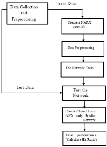
study is to use the NARX neural network for prediction while first the data preparation and then pre-processing are done before the data is manipulated to train the network and to simulate. After this stage, network is trained by the LM algorithm and the best structure is selected. Then, the predicted values by the network, the prediction error, and network performance are calculated based upon the MSE. After network training for proper evaluation, inputs are divided into three categories of training, validation and testing. Network performance is calculated for these categories. Also, the NARX neural networks with closed loop and removal delay are created and the performance of these two networks are calculated.
After network training and testing by training data, data checking is used for prediction as the final test. Finally, predicted signals by the network and the percentages of correct signals are determined.
Figure 2. Structure of the model
Figure 2 shows the general structure of the model while it will be discussed in details in the following parts.
3. 2. Create a Nonlinear Autoregressive Network
with External Input At this stage, the basic structure of the NARX neural network includes input delays, feedback delays, and hidden layer size which are determined and the NARX network is created on the basis of the specified values.
3. 2. 1. Data Pre-processing
3. 2. 1. 1. Prepare the Data for Training and Simulation In this step, the input time series are prepared for simulation or training of the network. Before preparation, the data are converted to a standard neural network format. Time-series data is converted from a matrix representation to standard cell array representation. Here data is defined in standard neural network data cell form. Converting this data does not change it [23].
Also, each time a network is transformed with open loop, close loop, remove delay or add delay, this function can reformat the data accordingly [25].
3. 2. 1. 2. Data Pre-processing Data quality is a
critical issue in prediction. To increase the accuracy of the prediction, we may perform data pre-processing techniques such data transformation [26]. Data preprocessing is an essential step in working with any ANNs [16].
Using transformed data is more useful in most heuristic methods especially when dealing with forecasting problems. A pre-processing method should contain the capability of transforming pre-processed data into its original scale (called post-processing).
One of the most useful data transformation techniques is data normalization. There are different
normalization algorithms, such as Min–Max
normalization, Z-score normalization, and sigmoid normalization. In this paper, we use Min–Max normalization which is a common approach in this field. The Min–Max normalization scales the numbers in a data set to improve the accuracy of the subsequent numeric computations. If Xold, Xmax, Xmin are the original, maximum and minimum values of the raw data, respectively and Xmax, Xmin, are the maximum and minimum of the normalized data, respectively, then the normalization of Xold called Xnew, can be obtained by the following transformation function [27]:
X
X
X
X X
X X
X old
new
* min *
min * max min max
min ( )
(6)
As a method to evaluate the usefulness of the model, we observe the results that calculate the difference in price between the result of the model and real target after a time unit. In this study for short-term forecasting of stock price movements, a 6-day stock market movement is used as the evaluation time unit. The price difference after 6 days indicates whether the model is successful or not. The Hit Ratio is defined as:
Successes of
Number Total
Successes of
Number
HitRatio (7)
If the Hit Ratio of the pattern is 51% or larger, the model can be approved. It means that investment according to the rule can result in a good profit [5].
3. 2. 3. Train and Test the Network The network is trained by the selected training function and the best structure of the network is selected. For the test network, MSE, as a performance function is calculated by the target data and outputs and prediction error, are also identified. To test the network, the network performance is calculated by test, validation and training data.
3. 2. 4. Closed Loop Network and Early Prediction Network In this stage, a close loop NARX network is created. The close loop converts neural network open-loop feedback to a closed one. The function replaces the feedback input with a direct connection from the out layer. This function takes a neural network and closes any open-loop feedback. In this stage, closed Loop Performance is calculated.
Furthermore, another neural network is created for remove delay. Remove delay returns the network with input delay connections that are decreased, and the output feedback delays that are increased, by the specified number of delays, n. The result is a network which behaves identically, except that outputs are produced in n time steps later. In this stage, early Prediction Performance is calculated.
3. 2. 5. Test Net with Testing Data Checking
data are used to test the trained neural network and the predicted values or network output is obtained.
3. 2. 6. Calculate Hit Ratio Finally, buy and sell signals and their total number are determined and correct signals are calculated during a 6-days period. By these obtained values, Hit Ratio as the main performance criteria is computed.
The semi-codes of the model are as follows: (1) Load data (Train Data and Test Data)
(2) Create a Nonlinear Autoregressive Network with External Input
Specifying Network Architecture: Input Delays, Feedback Delays, Hidden Layer Size create an NARX network
(3) Choose Input and Feedback Pre/Post-Processing Functions
(4) Prepare the Data for Training and Simulation (5) Setup Division of Data for Training, Validation, Testing
(6) Choose a Training Function Choose Levenberg-Marquardt; (7) Choose a Performance Function
Choose Mean Square Error(MSE);
(8) Train the Network: Training Neural Network using Levenberg - Marguardt Algorithm
(9) Test the Network
Calculate outputs
Calculate errors
Calculate network performance
Plot error of train data
Recalculate training, validation and test
(10) View the Network
(11) Create closed loop AND early predict network
Closed Loop Performance
(12) Early prediction network
Early Prediction Performance
Identify buy and sell signals and calculate Total number of signals
Calculate number of correct signals (success)
Calculate Hit Ratio
4. RESULTS AND DISCUSSION
4. 1. Input Data In this study the training data are
based upon two applied approaches of Jasemi et al. [28]. Applied approach for input is shown in Figure 3. The first approach (Raw database) is based on raw input features including 15 items and 1 output. In this approach the focus is on open (Oi), high (Hi), low (Li) and close (Ci) prices of the stock in the ith day due to the Japanese candlestick during last 3 days while to cover the stock price trend the close prices of the stock during the last 7 days are also included. The second approach (Signal based) is based on the reverse signals of Japanese candlestick technique including 24 input features and 1 output. This package covers the important factors of decision making in the technique. These approaches in 48 data sets are applied to train and test the introduced model that are past daily data of General Motors stocks in NYSE. Every input data is divided into two categories of training data and testing data. For more detail about input data refer to the study of Jasemi et al. [28].
4. 2. Experiment Results The input data of our experiments are daily stock prices of General Motors Company at New York Stock Exchange from 2000 to 2009. 48 datasets are applied for learning and checking. In this study, input Delays, feedback Delays and hidden Layer Size, 1:2, 1:2, 30 is considered, respectively. Division of data for Training, Validation, Testing are 70%, 15%, 15% respectively and the numbers of train epochs are considered to be 100.
The goal is to develop NARX model for TA approach. First, the training data is loaded. A tapped delay line is used with two delays for both the input and the output, so training begins with the third data point. The series-parallel NARX network is created.
Figure 3. The general approach in this model
Figure 4. NARX neural network with Raw Database
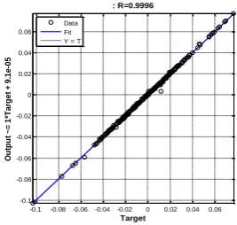
Figure 5. The linear regression of targets relative to outputs
30 neurons are used in the hidden layer and train LM is used for the training function, and then data is prepared. After training, the result is displayed in Figure 4. Figure 4 shows NARX neural network for the Raw approach as a graphical diagram. This structure is the same in NARX neural network for the Signal approach and only the number of input is different.
After completing parameters estimation validating the results against another set of data is necessary. For this purpose data was divided into three sets.
As mentioned before, MSE is used as the performance criteria. Network performance is calculated for signal approach and raw approach by training, validation, data testing and also data checking. Network performance is great and MSE value is low. Thus, the prediction accuracy is extremely high.
The linear regression between the network output and the actual output is calculated and is plotted for all data sets. Figure 5 shows this plot for data set 1 of Raw database (2000 for training and 2001 for checking) as an example. The linear regression value is 0.9996 for this data set and the regression model among these two variables is as follows:
5 . 0 1 . 9 arg
1
T et e
Output (8)
A histogram plot with normal fit for error of training data is another output of the model; this plot is shown in Figure 6 for data set 1. This plot is also shown in Figure 7 for error of checking of the data. The model plots a histogram of the values in the vector data using specified number of bins then superimposes a fitted normal distribution.
-0.1 -0.08 -0.06-0.04 -0.02 0 0.02 0.04 0.06 -0.1
-0.08 -0.06 -0.04 -0.02 0 0.02 0.04 0.06
Target
O
u
tp
u
t
~
=
1
*T
a
rg
e
t
+
9
.1
e
-0
5
: R=0.9996
It can be seen that the errors are very small. However, because of the series-parallel configuration, these are errors for only a one-step-ahead prediction. A more stringent test would be to rearrange the network into the original parallel form (closed loop) and then to perform an iterated prediction over many time steps. The structure of this network is shown in Figure 8.
Figure 6. Histogram with normal fit to the error of prediction
Figure 7. Histogram with normal fit to the error of prediction
Test data
Figure 8. NARX neural network (close loop) with Raw
databased
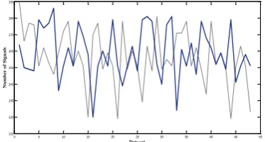
Figure 9. The total number of signals that are produced by
the approaches for each dataset
TABLE 1. The final result in comparison with other
prediction model
Total Hit Ratio
Hit Ratio Approach 1
Hit Ratio Approach 2
Supervised Feed
Forward NN [26] 74.2% 74.8% 73.6%
Wrapper
ANFIS-ICA [27] 86% 85% 87%
NARX NN 89% 89% 89%
Furthermore, by remove delay, the NARX network is used to predict the next output a time step (one step) ahead of when it will actually appear. Here, minimal tap delay is now 0 instead of 1.
In this study like Lee and Jo [5] and Jasemi et al. [28], a six-day stock market movement as the evaluation time unit is decided; that is each time a bull signal is followed by an actual upturn or a bear signal is followed by an actual downturn within 6 days; the signal is considered as a success. The correct signals are achieved by comparing the predictions with real happenings of the stock market. The complete list of the results is shown in appendix A. Figure 9 shows the total number of identified signals by the two approaches in different datasets. By the help of this figure, it can be verified that which of these approaches are better.
Lee and Jo [5] believe that if the hit ratio is above 51%, the model is regarded as useful and feasible. The total hit ratio of our new model is 89% while raw and signal data-based approaches have a hit ratio of 89% and are both equally successful.
The Number of identified signals by raw and signal approaches are shown in Figure 9. The correct percentage prediction for a 1 day period is shown as 0.32 and 0.33 for raw and signal approaches, respectively. In comparison with Jasemi et al.‟s study [28], our model is much better. The hit ratio of Jasemi et al.‟s model is 74.2% while this value in our model is 89% and this result is excellent. The Two approaches are equally successful in the current study while in the study by Jasemi et al. [28], the raw approach was better than the other approach.
5. CONCLUSION
In this paper, a new approach for modeling of TA by neural networks on the basis of the ancient investment technique of Japanese Candlestick is employed. NARX is used as an RNN while long-term dependencies exist. Although embedded memory can be found in all the recurrent networks, it is explained that why it is particularly prominent in NARX models.
Two approaches are used as input to the NARX neural network on the basis of the Japanese Candlestick
-10 -8 -6 -4 -2 0 2 4 6 8 10
0 10 20 30 40 50 60 70 80 90
Prediction Errors X 1000
n
u
m
b
e
r
o
f
b
in
s
normal distribution to the error Of prediction Train data
-15 -10 -5 0 5 10 15
0 20 40 60 80 100 120 140 160 180
Prediction Errors X 1000
n
u
m
b
e
r
o
f
b
in
s
normal distribution to the error Of prediction Test data
0 5 10 15 20 25 30 35 40 45 50
110 120 130 140 150 160 170 180 190
Data set
N
u
m
b
e
r
o
f
S
ig
n
a
charts patterns. These two approaches are studied in 48 different datasets with different training and checking periods and NARX neural network predictions. For this TA, the NARX neural network operates as an analyzer. Finally, the number of buy and sell signals and their correctness percentage is calculated.
In this study, the NARX neural network is examined on the basis of two criteria of hit ratio and MSE. According to the experimental results, it is proved that the network performance is excellent and better than the feed-forward static neural network. Moreover, the new model has a better hit ratio than the basic study of Jasemi et al. [28]. On the other hand, the Raw-based and signal-based approaches have similar performances with no significant difference between recognition of the buy and sell signals.
6. REFERENCES
1. Jasemi, M. and Kimiagari, A. M., "An investigation of model selection criteria for technical analysis of moving average",
Journal of Industrial Engineering International, Vol. 8, No. 1, (2012), 1-9.
2. Chavarnakul, T. and Enke, D., "A hybrid stock trading system for intelligent technical analysis-based equivolume charting",
Neurocomputing, Vol. 72, No. 16, (2009), 3517-3528. 3. Marshall, B. R., Young, M. R. and Rose, L. C., "Candlestick
technical trading strategies: Can they create value for investors?", Journal of Banking & Finance, Vol. 30, No. 8, (2006), 2303-2323.
4. Kamo, T. and Dagli, C., "Hybrid approach to the japanese candlestick method for financial forecasting", Expert Systems with applications, Vol. 36, No. 3, (2009), 5023-5030.
5. Lee, K. and Jo, G., "Expert system for predicting stock market timing using a candlestick chart", Expert Systems with Applications, Vol. 16, No. 4, (1999), 357-364.
6. Xie, H., Zhao, X. and Wang, S., "A comprehensive look at the predictive information in japanese candlestick", Procedia Computer Science, Vol. 9, (2012), 1219-1227.
7. Lan, Q., Zhang, D. and Xiong, L., "Reversal pattern discovery in financial time series based on fuzzy candlestick lines", Systems Engineering Procedia, Vol. 2, (2011), 182-190.
8. Chen, Y., Mabu, S. and Hirasawa, K., "A model of portfolio optimization using time adapting genetic network programming", Computers & Operations Research, Vol. 37, No. 10, (2010), 1697-1707.
9. Crone, S. F. and Kourentzes, N., "Feature selection for time series prediction–a combined filter and wrapper approach for neural networks", Neurocomputing, Vol. 73, No. 10, (2010), 1923-1936.
10. Chang, P.-C., "A novel model by evolving partially connected neural network for stock price trend forecasting", Expert Systems with Applications, Vol. 39, No. 1, (2012), 611-620. 11. Atsalakis, G. S., Dimitrakakis, E. M. and Zopounidis, C. D.,
"Elliott wave theory and neuro-fuzzy systems, in stock market prediction: The wasp system", Expert Systems with Applications, Vol. 38, No. 8, (2011), 9196-9206.
12. Pradeep, J., Srinivasan, E. and Himavathi, S., "Neural network based recognition system integrating feature extraction and
classification for english handwritten", International Journal of Engineering-Transactions B: Applications, Vol. 25, No. 2, (2012), 99-106.
13. Lin, X., Yang, Z. and Song, Y., "Intelligent stock trading system based on improved technical analysis and echo state network",
Expert Systems with applications, Vol. 38, No. 9, (2011), 11347-11354.
14. Lee, M.-C., "Using support vector machine with a hybrid feature selection method to the stock trend prediction", Expert Systems with Applications, Vol. 36, No. 8, (2009), 10896-10904. 15. Huang, S.-C. and Wu, T.-K., "Integrating ga-based time-scale
feature extractions with svms for stock index forecasting",
Expert Systems with Applications, Vol. 35, No. 4, (2008), 2080-2088.
16. O‟Connor, N. and Madden, M. G., "A neural network approach to predicting stock exchange movements using external factors",
Knowledge-Based Systems, Vol. 19, No. 5, (2006), 371-378. 17. Goel, A., "Ann based modeling for prediction of evaporation in
reservoirs (research note)", International Journal of Engineering-Transactions A: Basics, Vol. 22, No. 4, (2009), 351-358.
18. Mahmoud, S., Lotfi, A. and Langensiepen, C., "Behavioural pattern identification and prediction in intelligent environments",
Applied Soft Computing, Vol. 13, No. 4, (2013), 1813-1822. 19. Andalib, A. and Atry, F., "Multi-step ahead forecasts for
electricity prices using narx: A new approach, a critical analysis of one-step ahead forecasts", Energy Conversion and Management, Vol. 50, No. 3, (2009), 739-747.
20. Pisoni, E., Farina, M., Carnevale, C. and Piroddi, L., "Forecasting peak air pollution levels using narx models",
Engineering Applications of Artificial Intelligence, Vol. 22, No. 4, (2009), 593-602.
21. Kim, H.-j. and Shin, K.-s., "A hybrid approach based on neural networks and genetic algorithms for detecting temporal patterns in stock markets", Applied Soft Computing, Vol. 7, No. 2, (2007), 569-576.
22. Huo, F. and Poo, A.-N., "Nonlinear autoregressive network with exogenous inputs based contour error reduction in CNC machines", International Journal of Machine Tools and Manufacture, Vol. 67, (2013), 45-52.
23. Sahoo, H., Dash, P. and Rath, N., "Narx model based nonlinear dynamic system identification using low complexity neural networks and robust h∞ filter", Applied Soft Computing, Vol. 13, No. 7, (2013), 3324-3334.
24. Ardalani-Farsa, M. and Zolfaghari, S., "Chaotic time series prediction with residual analysis method using hybrid elman– narx neural networks", Neurocomputing, Vol. 73, No. 13, (2010), 2540-2553.
25. Soman, P. C., "An adaptive narx neural network approach for financial time series prediction", Rutgers University-Graduate School-New Brunswick, (2008),
26. Asadi, S., Hadavandi, E., Mehmanpazir, F. and Nakhostin, M. M., "Hybridization of evolutionary levenberg–marquardt neural networks and data pre-processing for stock market prediction",
Knowledge-Based Systems, Vol. 35, (2012), 245-258. 27. Atsalakis, G. S. and Valavanis, K. P., "Surveying stock market
forecasting techniques–part ii: Soft computing methods", Expert Systems with applications, Vol. 36, No. 3, (2009), 5932-5941. 28. Jasemi, M., Kimiagari, A. M. and Memariani, A., "A modern
neural network model to do stock market timing on the basis of the ancient investment technique of japanese candlestick",
7. Appendix A
Table A 1: The complete list of the results is brought here. The columns of 1 to 6, column 7 and column 8 show the correct signals in 1, 2, 3, 4, 5, and 6 day periods, the total number of correct signals and the total number of the emitted signals by the system, respectively.
TABLE A 1. The complete list of the results
Raw Data base
8 7 6 5 4 3 2 1 No 190 181 9 13 20 29 42 68 1 166 155 9 13 19 21 46 47 2 177 159 1 5 17 22 46 68 3 176 163 8 14 14 18 43 66 4 151 134 7 8 12 15 41 51 5 162 139 10 13 15 20 31 50 6 153 133 10 11 11 20 31 50 7 146 117 6 9 17 22 28 35 8 159 150 8 13 19 18 45 47 9 172 156 1 4 17 22 45 67 10 178 165 8 14 15 18 43 67 11 151 133 7 10 12 15 39 50 12 160 139 10 13 15 20 31 50 13 151 134 10 11 13 21 33 46 14 120 103 3 7 12 20 25 36 15 170 154 1 3 17 22 45 66 16 177 164 8 14 15 18 43 66 17 149 139 8 12 12 16 42 49 18 159 138 10 13 15 20 31 49 19 151 134 12 12 12 18 32 48 20 119 101 3 7 13 20 25 33 21 178 165 8 14 15 18 43 67 22 149 132 7 10 11 15 40 49 23 160 138 10 13 15 20 31 49 24 151 126 10 11 11 17 30 47 25 129 106 5 7 14 21 23 36 26 163 156 9 14 19 21 46 47 27 148 135 7 8 14 25 37 44 28 181 167 8 15 15 18 43 68 29 149 132 7 9 11 15 40 50 30 155 133 10 11 13 21 30 48 31 151 127 10 11 10 19 30 47 32 171 137 7 13 17 23 34 43 33 171 155 1 4 17 22 45 66 34
Raw Data base
8 7 6 5 4 3 2 1 No 178 165 8 14 15 18 43 67 35 151 134 7 10 12 15 40 50 36 162 147 11 14 16 22 32 52 37 149 125 10 11 11 17 30 46 38 134 109 6 7 14 21 25 36 39 178 165 8 14 15 18 43 67 40 152 147 3 5 12 21 42 64 41 159 138 10 13 15 20 31 49 42 150 126 10 11 11 18 30 46 43 119 96 3 6 12 18 23 34 44 150 132 7 10 11 15 40 49 45 163 140 10 13 16 20 32 49 46 151 127 10 11 11 18 30 47 47 123 100 3 6 13 18 25 35 48
Signal Data base
A Nonlinear Autoregressive Model with Exogenous Variables Neural Network for
Stock Market Timing: The Candlestick Technical Analysis
E. Ahmadia, M. H. Abooiea, M. Jasemib, Y. Zare Mehrjardia
a Department of Industrial Engineering, Yazd University, Yazd, Iran
b Department of Industrial Engineering, Khajeh Nasir Toosi University of Technology, Tehran, Iran
P A P E R I N F O
Paper history:
Received 19 February 2015
Received in revised form 09 September 2016 Accepted 08 October 2016
Keywords: Finance
Stock Market Forecasting Technical Analysis
NARX Recurrent Neural Network Levenberg–marquardt Algorithm
ديكچ ه
راخ یاَریغتم اب یطخریغ ًیسرگرًتا لدم ،ٍلاقم هیا رد ماُس یاَرازاب یدىب نامز یارب دیدج یبصع ٍکبض کی ناًىع ٍب یج
.تسا رگ لیلحت کی یجراخ یاَریغتم اب یطخریغ ًیسرگرًتا ،لدم رد .تسا ٍتفر راک ٍب یىپاژ نادعمض یىف لیلحت ساسا رب عت یديري یاَ ٌداد داجیا یارب لاىگیس ي ماخ یاَداد رب یىتبم درکیير يد )تایبدا دىوامَ( اجىیا تحص دصرد .دوا ٌدض ٍیب
یوامز یاَ ٌريد یارب یىیب صیپ 1
-6 یم تابثا جیاتو .تسا ٌدض ٍتفرگ رظو رد شيرف ي دیرخ یاَ لاىگیس لک دادعت اب ٌزير
ٌدض داجیا ٍکبض .دوراد یرترب يرطیپ یبصع ٍکبض زا اَ نآ ٍک یلاح رد دوراد یا ٍباطم درکلمع یدح ات اَدرکیير ٍک دىک ایم رایعم طسًت .تسا ٌدض ٍبساحم لااب رایسب یىیب صیپ لدم تحص ي دًض یم یبایزرا اطخ عبرم هیگو