Please cite this article as: Z. Sheikh Khozani, H. Bonakdari, A. H. Zaji, Comparison of Three Soft Computing Methods in Estimating Apparent Shear Stress in Compound Channels, International Journal of Engineering (IJE), TRANSACTIONSC: Aspects Vol. 29, No. 9, (September 2016) 1219-1226
International Journal of Engineering
J o u r n a l H o m e p a g e : w w w . i j e . i rComparison of Three Soft Computing Methods in Estimating Apparent Shear Stress
in Compound Channels
Z. Sheikh Khozani, H. Bonakdari*, A. H. Zaji
Department of Civil Engineering, Razi University, Kermanshah, Iran
P A P E R I N F O
Paper history:
Received 26 February 2016 Received in revised form 16 July 2016 Accepted 25 August 2016
Keywords: Apparent Shear Stress Multi Layer Perceptron Radial Basis Function Genetic Programing
Genetic Algorithm Artificial Neural Network Decision Tree
Symmetric Compound Channel
A B S T R A C T
Apparent shear stress acting on a vertical interface between the main channel and floodplain in a compound channel serves to quantify the momentum transfer between sub sections of this cross section. In this study, three soft computing methods are used to simulate apparent shear stress in prismatic compound channels. The Genetic Algorithm Artificial neural network (GAA), Genetic Programming (GP) and Modified Structure-Multi Layer Perceptron (MS-MLP) are applied to about 100 different data to predict apparent shear stress. The modelling procedure with three models were extended and the best of each model was selected after each step. In modeling with the GAA and GP different input combinations, fitness functions, transfer functions and mathematical functions were investigated for obtaining the optimum combination. The results showed B/b, H/B, nf/nc and h/b as
input combination, fitness function MSE and transfer function tan-pur is the best combination for GAA model. The best GP model introduced with B/b, (H-h)/h, nf/nc and h/b as input variables, fitness
function MAE and
,,,,sin,cos,abs,sqrt,power
as the mathematical function set. Finally, the most appropriate GAA, GP and MS-MLP models were compared to select the best of them in estimating apparent shear stress in compound channels. According to the results, MS-MLP improved with RMSE of 0.3654 over GAA with RMSE of 0.5326 and the GP method with RMSE of 0.6615.doi: 10.5829/idosi.ije.2016.29.09c.06
1. INTRODUCTION1
A compound cross section is the most common section in natural rivers and consists of a floodplain which is rougher and wider than the main channel. If flooding occurs, the characteristics of river flow are more complicated than in normal mode due to the variations in geometry and roughness between the main channel and floodplain. Flow resistance also increases due to the transverse momentum transfer, which consumes the flow’s kinetic energy as well. By ignoring the effect of momentum transfer, the results of models that estimate discharge in compound channels would not be as reliable as with traditional discharge predictions. Myers [1] showed that apparent shear stress (τa) is an essential
parameter in transverse momentum transfer. Therefore,
1*Corresponding Author’s Email: bonakdari@yahoo.
com (H. Bonakdari)
Therefore, investigating other methods that can predict apparent shear stress without the need for these parameters is a novel concept.
Using soft computing (SC) methods for predicting different hydraulic phenomena is an ongoing endeavor [7-9]. Huai et al. [10] investigated application of Artificial Neural Network (ANN) in predicting apparent shear stress in compound channels with and without vegetation. Sheikh Khozani et al. [11] employed GP and GAA methods to predict percentage of shear force carried by walls in rough rectangular channel.
In this study, three SC methods (GAA, GP and MS-MLP) are applied to estimate the apparent shear stress in prismatic compound channels with smooth and rough boundaries. After extending the models, their results are compared to select the most appropriate model in predicting apparent shear stress in prismatic compound channels. Therefore, only with the knowledge of channel geometry and roughness the apparent shear stress can be calculated using best model with acceptable accuracy.
2. MATHEMATICAL AND METHODS
2. 1. Experimental Data Used To predict apparent shear stress in symmetric compound channels with smooth and rough boundaries, about 100 experimental data were collected from different studies of Knight and Hamed [3], Prinos and Townsend [4], Knight and Demetriou [12], and Wormleaton and Merrett [13]. These data were collected of small-scale flume data and large-scale Flood Channel Facility (FCF). According to the results of several researchers, the effective parameters in apparent shear stress values are introduced as: channel height (H), total width (B), main channel width (b), main channel flow depth (h),, flood plain roughness (nf) and main channel roughness
(nc). So, the apparent shear stress in compound channels
is a function of:
f c
aFH,h,B,b,n ,n
(1)
After applying Buckingham’s theorem, the six dimensionless parameters which used in modeling obtained as:
bh BH B H b h h
h H n n
b B f
c f
a , , , , ,
(2)
2. 2. GAA Modeling One of the most used methods for solving complex engineering problems, is ANN model. This model consists of an input layer, an output layer and one or more hidden layer. The neuron number of the input and output layers is the same as the number of input and output variables, respectively. The neuron number of hidden layer is not specified so the trial and error method was used to find the appropriate
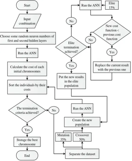
number of hidden layer [14]. However, this method is time consuming. In this study, a modified GA was made to optimizethe ANN model structure and identify the neuron numbers of each hidden layer. The flowchart of the introduced GAA is shown in Figure 1.
GA algorithm requires some modification to become proper to optimize the ANN structure, since the random nature of the Levenberg-Marquardt Algorithm [15] in weights and bias determination, it is probable that an appropriate individual was put out from the GAA resulted in bad luck in this algorithm process. To solving this problem, a modification was applied in the elite population of the GA approach. The GA method was applied to run the elite population several times to find the best cost of each chromosome and then transfer the chromosomes to the next generation. By these modifications of the chromosomes of the elite population, they are not simply changed but are lead to avoid the GAA method from trapping in the local minimums and also successful the random nature of the Levenberg-Marquardt algorithm.
The GAA has several parameters which should be initially determined to model. The GAA includes two runs: the MLP-ANN and the GA. The number of termination period of MLP-ANN runs was considered 100, so the models completely converge. The GA mutation and crossover frequency considered are 35% and 50%, respectively, therefore the models performed well. The GA population size intended is 30, and the termination criterion intended is 100 generations without result improvement.
Figure 1. GAA flowchart
Start
Input combination
Choose some random neuron numbers of first and second hidden layers
Run the ANN
Calculate the cost of each initial chromosomes
Sort the individuals by their costs
The termination criteria achieved?
Storage the best chromosome
End Yes
No
Separate the dataset Mutation
35%
Crossover 50%
Elite 15%
Create the new population Run the ANN
Run the ANN
New cost function < previous cost
function
Replace the current result with the previous one
Yes No
Elite termination
achieved?
Put the new results in the elite population
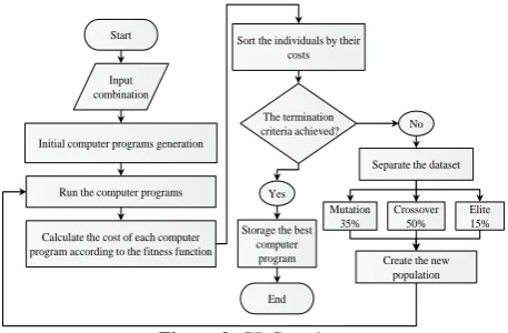
2. 3. GP Modeling The GP method [16], a subset of GA, is widely employed in different engineering problems. In the GP method, individuals are the computer programs. The GP process starts with a random initial population of computer programs. Each computer program is formed randomly in accordance with user-determined parameters, such as initial program size and mathematical functions that a computer program is permitted to use. Then, the cost of each program is computed using the fitness function, and the GP process serves to determine the best computer program which can simulate the considered problem. The GP flowchart is presented in Figure 2.
It is obviously seen that similar to the GA, the crossover, mutation and elite processes occur in the GP method as well. In crossover, two individuals from the current generation are selected, and two chromosomes are generated for the next generation through the crossover procedure. Mutation is in order to maintain genetic diversity between GP generations. The best computer program of each generation is saved as the elite population, which is directly moved to the next generation.
2. 4. MS-MLP Modeling Applying the DT algorithm [17] rather than a similar allocation of the MLP power on the entire dataset, this method is fragmented into the same models. The dataset is then divided into smaller datasets, and the smaller models are employed to model the separated datasets.
The advantage of the DT-based MLP method is the reallocation of the whole power of the artificial intelligence method to the divided dataset segments. The following steps are performed in the DT-based MLP method.
(a) The entire dataset is divided to smaller of them. In this study, according to the apparent shear stress amounts, the dataset is divided into the LOW, MEDIUM, and HIGH apparent shear stress groups. (b) Now, the DT is divided into testing and training datasets and in training dataset starts to estimate dataset
Figure 2. GP flowchart
group (LOW, MEDIUM, or HIGH) using the input parameters. If the accuracy division is weak, the simpler DT structure is obtained; but, the errors increase. The weak division accuracy has the advantage of a simpler DT structure, but the division error is high. The higher accuracy DT algorithm increases the accuracy of predicting, but it lead to s: over fitting and the large DT structure. Thus, the trial and error method is applied to determine the DT algorithm precision.
(c) The artificial intelligence method applied is split into smaller models. In this study, 12-hidden-neuron MLP models were utilized. Therefore, each of these models is split into three, four-neuron models.
(d) The divided datasets are modeled using the smaller MLP models. The number of hidden neurons in each smaller model is specified using trial and error. It is obvious that for each smaller model, the maximum permissible number of hidden neurons is 4.
(e) The results of separated, smaller models are cumulated into one united model.
2. 5. Model Performance Evaluation statistical parameters are employed as: the coefficient of correlation (R), the Root Mean Square Error (RMSE), the mean square error (MSE) and the Mean Absolute Error (MAE). These statistical parameters are defined as follow:
n
i
n
i
ip ip im
im n
i
ip ip im im
x x x
x
x x x x
R
1
2
1 2 1
(3)
n x x
RMSE
n
i
im ip
1
2
(4)
n MSE
n
i
im ip
1
2
(5)
n
i
im
ip
x
x n MAE
1
1
(6)
where, xip is the estimated apparent shear stress by
models, xim is the apparent shear stress measured in the
laboratory and n is the number of data.
3. RESULTS AND DISSCUSION
3. 1. Input Selection Selecting the best input combination is an important step in modeling with SC methods. Also, selecting the best input combination avoids the model from entering wrong input data that would obscure the training process. This step leads to
Start
Input combination
Initial computer programs generation
Run the computer programs
Calculate the cost of each computer program according to the fitness function
Sort the individuals by their costs
The termination criteria achieved?
Storage the best computer
program
End Yes
No
Separate the dataset
Mutation 35%
Crossover 50%
Create the new population
increase model precision in estimating output data. In modeling with MS-MLP method for select the best input combination, this step was applied in simple MLP and the best input combination selected was used in modeling with MS-MLP model. To select the most appropriate input parameters, four different input combinations were studied as follows:
b h n n
h h H b B
c f
, , , :
1
b h
n n
B H
b B
c f
, , , : 2
c f
n n
h H b B
, , : 3
c f n n
bh BH , : 4
where, H is channel height, h is main channel flow depth, B is total width, b is main channel widths, nf and
nc flood plain and main channel roughness, respectively.
The results of this step are shown in Figure 3. According to this figure, none of the three mentioned methods could estimate the apparent shear stress with input combinations (3) and (4). The worst results with lower accuracy were obtained when the input combinations (3) and (4) were used. It shows ignoring input variable h/b had been more influence in results. Therefore, this parameter is important in modeling of apparent shear stress. The GAA method showed the best performance with using input combination (2) which resulted in predicting apparent shear stress with sufficient accuracy. The GP and MS-MLP methods using input combinations (1) and (2) respectively showed better performance with lower statistical parameters than those of other input combinations. It can be deducted parameter H/B in modeling with MS-MLP and GAA models help model to increase accuracy of predictions. Also, in modeling with GP model parameter (H+h)/h influences in increasing model precision.
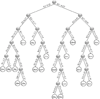
3. 2. Hybrid DT-based Neural Network To improve the results, the MS-MLP model is used in this section keeping in view input combination (2). After the trial and error procedure (according to the second step in the DT-based method mentioned before), the structure of the optimum DT is illustrated in Figure 4. In this figure, x1, x2, x3, and x4 represent the input variables B/h, H/h, nf/nc and h/b, respectively.
The results of modeling with MS-MLP are illustrated in Figure 5. It is seen that this model could predict close results to experimental data. As seen from the fitted line equation (assuming the equation is
y=a1x+a2), in the scatter plot the a1 coefficients is very
close to 1 and a2 is close to 0. This indicates that the
values predicted by this equations is more accurate.
Figure 3. Statistical parameter of input combination selection for models for test dataset
Figure 5. Scatter plot of observed and predicted apparent shear stress using MS-MLP method
Also, the coefficient of correlation is very high and it confirms the high precision of model to predict apparent shear stress in compound channels.
3. 3. Selecting the Most Appropriate Fitness Function The second step in modeling with GP and GAA is to select the best fitness function. For this aim, the MSE and MAE fitness functions are investigated. Based on the results in Table 1, for modeling with GAA, the MSE fitness function with RMSE of 0.533 indicated better performance than MAE with RMSE of 0.542. It is noted that input combination (2) was used in modeling with GAA. In modeling with the GP method and using input combination (1) as the best input combination, the MAE fitness function with the lowest statistical parameter value demonstrated better performance than the MSE fitness function. Therefore, the MSE and MAE fitness functions were selected in modeling with GAA an GP methods respectively for next step.
3. 4. Selecting the Transfer Function The last step in modeling with the GAA method is selecting the most suitable transfer function. Selecting a suitable transfer function for the hidden and output layers directly influences multilayer perceptron neural network performance. Therefore, different combinations of logarithmic, hyperbolic tangent and linear transfer functions (Equations (7)-(9)) are applied and compared for the GAA method.
TABLE 1. Fitness function selection for the GAA and GP methods
Models GAA Model GP Model
Fitness Function MSE MAE MSE MAE
RMSE 0.533 0.542 0.665 0.662 MAE 0.381 0.387 0.477 0.453 R 0.980 0.980 0.966 0.967
x e x logsig 1 1 ) ( (7) 1 1 2 )
( 2
x
e x
tansig (8)
x x
purelin( ) (9)
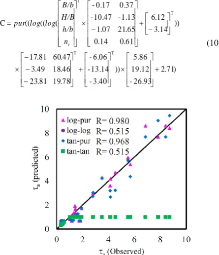
The results of this step are shown in Figure 6. It is evident that applying similar transfer functions in the input and output layers, such as tan-tan or log-log, decreases the precision of apparent shear stress estimation. However, selecting different transfer functions in the output and input layers significantly increases the precision of the estimated values with R of 0.980 for the logarithmic and purelin functions in the input and output layers, respectively, and R of 0.968 for
tan-pur as the transfer function. Hence, in the GAA model, the logarithmic transfer function in the hidden layer and purlin transfer function in the output layer demonstrated the best performance with high accuracy in all situations. As seen in this figure, when using log-log or tan-tan transfer functions, the predicted apparent shear stress values are somewhat constant at all flow depths. Moreover, underestimated values were produced and all predictions were around the straight line. It can be deducted that if the transfer functions tan-tan and
log-log are used in the modeling process, the results are not accurate or reliable.
Equation (10) was obtained for computing the apparent shear stress with the most appropriate GAA model with input combination (2), MSE fitness function and log-pur transfer function as:
) 71 . 2 26.93 -19.12 5.86 )) 3.40 -13.14 -6.06 -78 . 19 81 . 23 46 . 18 49 . 3 47 . 60 81 . 17 )) 14 . 3 12 . 6 61 . 0 14 . 0 65 . 21 07 . 1 1.13 -10.47 -0.37 0.17 -( (( (( C T T T T r n h/b H/B B/b log log pur (10)
3. 5. Selecting the Mathematical Functions The final step in modeling with GP is selecting the best mathematical function set. A function combination is selected based on the simplicity or complexity of the computer programs. Equations (11) to (14) represent that the first function combination uses the simplest mathematical function and by moving from the first function combination to the last, the model complexity increases.
, , ,
1
F (11)
, , , ,sin,cos
2
F (12)
abssqrtpower
F3 ,,,,sin,cos, , , (13)
, , , ,sin,cos, , , ,exp
4 abssqrt power
F (14)
According to the results in Figure 7, mathematical function set F3 with the highest R of 0.969 performed the best compared to the other mathematical function sets. It is noted that although the simplest function set
F1 showed good results, the results of the F3 mathematical function set were more accurate than those of other function sets. Thus, the GP model with input (1), MAE transfer function and function set
abssqrtpower
F3 ,,,,sin,cos, , , was selected as the most appropriate GP model for estimating the apparent shear stress in symmetrical compound channels.
The output of GP model is a program which illustrated in Box 1. As seen in this Box, the program is written as a MATLAB code which get input values and can predict the value of apparent shear stress.
3. 6. Comparison between the Most Appropriate Models All three SC methods, namely GAA, GP and MS-MLP are compared to identify the best model for estimating apparent shear stress. It is noted that in GAA modeling, input combination (2), fitness function MSE and transfer function log-pur were used.
Also, the best GP model utilized input combination (1), fitness function MAE and F3 as the mathematical
Figure 7. Scatter plot of the most suitable mathematical function selected for the GP model
Box 1. The output program of the best GP model
function set. Figure 8 illustrates the comparison between all models in predicting the apparent shear stress for the entire data set. As seen in this figure, all three models could predict apparent shear stress close to experimental data and their results were acceptable.
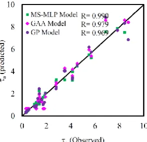
Figure 9 illustrates the scatter plot of all models employed with the test dataset.
Figure 8. Comparison between the MS-MLP, GAA and GP models as a hydrograph for the entire data set
Figure 9. Comparison between the MS-MLP, GAA and GP models as a scatterplot for the entire data set
V1=input('B/b = ');
V2=input('(H-h)/H = ');
V3=input('h/b = ');
V4=input('nf/nc = ');
C=0; a=0; C=C-0.0026; C=C/-1.642; C = C + V3; a=a+C; C=C*a; C=C+C; C=C*C; C=C+V1; C=cos(C); C=abs(C); C=C-V2; C=sin(C); C=C/a; C=abs(C); C=sin(C); C=C/0.634; C=C-a; C=C+1.987; C=C/a; C=sqrt(C); C=C-V2; C=C-V2; C=C-V2; C=C*V4; C=C+0.0327; C=C/-0.649; C=abs(C); C=C+0.131;
disp('The apparent shear stress
According to Figure 9, the MS-MLP model with R of 0.990 demonstrated the best performance in predicting apparent shear stress compared to the GAA and GP models with R of 0.979 and 0.969, respectively. Considering the R values of all three models, it can be deducted that all models estimated apparent shear stress values in compound channels accurately and can be used in place of traditional methods for calculating τa.
4. CONCLUSION
Since apparent shear stress is an important parameter in transverse momentum transfer that occurs between the main channel and floodplain in compound channels, estimating this parameter using MS methods was investigated in this study. According to the effective parameters on apparent shear stress values and after using Buckingham’s theorem, six dimensionless parameters were considered as input variables: B/b,
nf/nc, (H-h)/h, h/b, H/B and BH/bh. Then, four different
input combinations were applied to the GP, GAA and MS-MLP models to investigate the best input combinations.
In modeling with GP and GAA two fitness functions were studied, i.e. Mean Squared Error (MSE) and Mean Absolute Error (MAE). Modeling apparent shear stress with the GP method with B/b, nf/nc, (H-h)/h and h/b
selected as the input combination, MAE as the fitness function and the
,,,,sin,cos,abs,sqrt,power
mathematical function produced the best results withRMSE of 0.6615 for the test dataset compared to the other GP models. Among the GAA models applied to the data, the best model had B/b, nf/nc, H/B and h/b as
the input combination, MSE as the fitness function and the logarithmic transfer and purelin functions for the hidden and output layers, respectively. The best GAA model had RMSE of 0.5326 for the test dataset. The MS-MLP model with a similar input combination to the best GAA model had RMSE of 0.3654 and made the most appropriate predictions of apparent shear stress in compound channels.
Therefore, the MS-MLP model with higher apparent shear stress estimation precision was introduced as the best SC model for predicting this phenomenon. It is noted the results of GP and GAA models were so good and the proposed program and equations are more applicable. Also, using these methods can be used as alternative of traditional equations for estimating apparent shear stress which require knowledge of the velocity gradient.
5. REFERENCES
1. Myers, W., "Momentum transfer in a compound channel",
Journal of Hydraulic Research, Vol. 16, No. 2, (1978), 139-150.
2. Rajaratnam, N. and Ahmadi, R., "Hydraulics of channels with flood-plains", Journal of Hydraulic Research, Vol. 19, No. 1, (1981), 43-60.
3. Knight, D.W. and Hamed, M.E., "Boundary shear in symmetrical compound channels", Journal of Hydraulic Engineering, Vol. 110, No. 10, (1984), 1412-1430.
4. Prinos, P. and Townsend, R., "Comparison of methods for predicting discharge in compound open channels", Advances in Water resources, Vol. 7, No. 4, (1984), 180-187.
5. Rajaratnam, N. and Ahmadi, R.M., "Interaction between main channel and flood-plain flows", Journal of the Hydraulics Division, Vol. 105, No. 5, (1979), 573-588.
6. Moreta, P.J. and Martin-Vide, J.P., "Apparent friction coefficient in straight compound channels", Journal of Hydraulic Research, Vol. 48, No. 2, (2010), 169-177. 7. Sadeghpoor, M., "A wavelet support vector machine
combination model for daily suspended sediment forecasting",
International Journal of Engineering-Transactions C: Aspects, Vol. 27, No. 6, (2013), 531-540.
8. Mirzaei, E., Minatour, Y., Bonakdari, H. and Javadi, A., "Application of interval-valued fuzzy analytic hierarchy process approach in selection cargo terminals, a case study", (2015). 9. Bonakdari, H., Ebtehaj, I. and Azimi, H., "Numerical analysis of
sediment transport in sewer pipe", International Journal of Engineering-Transactions B: Applications, Vol. 28, No. 11, (2015), 1564.
10. Huai, W., Chen, G. and Zeng, Y., "Predicting apparent shear stress in prismatic compound open channels using artificial neural networks", Journal of Hydroinformatics, Vol. 15, No. 1, (2013), 138-146.
11. Sheikh Khozani, Z., Bonakdari, H. and Zaji, A.H., "Application of a soft computing technique in predicting the percentage of shear force carried by walls in a rectangular channel with non-homogeneous roughness", Water Science and Technology, Vol. 73, No. 1, (2016), 124-129.
12. Knight, D.W. and Demetriou, J.D., "Flood plain and main channel flow interaction", Journal of Hydraulic Engineering, Vol. 109, No. 8, (1983), 1073-1092.
13. Wormleaton, P. and Merrett, D., "An improved method of calculation for steady uniform flow in prismatic main channel/flood plain sections", Journal of Hydraulic Research, Vol. 28, No. 2, (1990), 157-174.
14. Kisi, O. and Kerem Cigizoglu, H., "Comparison of different ann techniques in river flow prediction", Civil Engineering and Environmental Systems, Vol. 24, No. 3, (2007), 211-231. 15. Levenberg, K., "A method for the solution of certain non-linear
problems in least squares", Quarterly of Applied Mathematics, Vol. 2, No. 2, (1944), 164-168.
16. Koza, J.R., "Genetic programming: On the programming of computers by means of natural selection, MIT press, Vol. 1, (1992).
Comparison of Three Soft Computing Methods in Estimating Apparent Shear Stress
in Compound Channels
Z. Sheikh Khozani, H. Bonakdari, A. H. Zaji
Department of Civil Engineering, Razi University, Kermanshah, Iran
P A P E R I N F O
Paper history:
Received 26 February 2016 Received in revised form 16 July 2016 Accepted 25 August 2016
Keywords: Apparent Shear Stress Multi Layer Perceptron Radial Basis Function Genetic Programing
Genetic Algorithm Artificial Neural Network Decision Tree
Symmetric Compound Channel
ديكچ ه
لاًاک رد یلصا لاًاک ٍ تضد بلایس يیت یدَوع ِحفص رد ِک یرّاظ یضرت صٌت یه لوع ةکره یاّ
يییعت یارت ،ذٌک
یه ُدافتسا اّ لاًاک يیا رد نتٌهَه لاقتًا لاًاک رد یضرت صٌت مرً تاثساحه شٍر ِس زا ُدافتسا ات ِلاقه يیا رد .دَض
یاّ
ةکره یه یٌیت صیپ ( کیتًژ نتیرَگلا یثصع ِکثض یاّ شٍر .دَض
GAA ( کیتًژ یسیًَ ِهاًرت ،) GP
ىٍرتپسرپ ٍ )
( ُذض حلاصا MS-MLP
صیپ یارت تٍافته ُداد ذص یٍر رت ) لذه ذٌیآرف .ذض لاوعا یرّاظ یضرت صٌت یٌیت
ات یزاس
ت .ذض باختًا ِلحره رّ رد لذه يیرتْت ٍ ذض ُدرتسگ شٍر ِس زا ُدافتسا لذه رد تلاح يیرتْت باختًا یار
ِت یزاس
شٍر GAA ٍ GP ةیکرت رارق یسررت درَه یفلتخه یضایر عتاَت ٍ شزارت عتاَت ،لاقتًا عتاَت ،تٍافته یدٍرٍ یاّ
لذه يیرتْت ،جیاتً ساسا رت .تفرگ GAA
ات B/b, H/B, nf/nc and h/b ،یدٍرٍ یاّریغته ىاٌَع ِت
MSE ىاٌَع ِت
ٍ شزارت عتات log-pur
آ تسد ِت لاقتًا عتات ىاٌَع ِت لذه يیرتْت .ذه
GP ات B/b, (H-h)/h, nf/nc and h/b ِت
شزارت عتات ،یدٍرٍ یاّریغته ىاٌَع MAE
یضایر عتاَت ٍ
,,,,sin,cos,abs,sqrt,power
يیرتْت ىاٌَع ِت
ٍ کیتًژ یسیًَ ِهاًرت ،کیتًژ نتیرَگلا یثصع ِکثض لذه يیرتْت ىایاپ رد .ذض یفرعه لذه ات ُذض حلاصا ىٍرتپسرپ
لذه يیت ٍ ُذض ِسیاقه رگیذکی جیاتً ساسا رت .ذض باختًا یرّاظ یضرت صٌت یٌیت صیپ رد لذه يیرتْت ُذض رکر یاّ
لذه MS-MLP ات
RMSE=0.3654 ِت تثسً
GAA ات RMSE=0.5326 ٍ
GP ات RMSE=0.6615 يیرتْت
.داد ىاطً یرّاظ یضرت صٌت یٌیت صیپ رد ار درکلوع