Numerical Study of Interaction of Two Plane Parallel Jets

Please cite this article as: N. Hnaien, S. Marzouk Khairallah, H. Ben Aissia, J. Jay, Numerical Study of Interaction of Two Plane Parallel Jets, International Journal of Engineering (IJE), TRANSACTIONS A: Basics Vol. 29, No. 10, (October 2016) 1421-1430

International Journal of Engineering

Numerical Study of Interaction of Two Plane Parallel Jets

N. Hnaien*a_{, S. Marzouk Khairallah}a_{, H. Ben Aissia}a_{, J. Jay}b

a _{Unite of Metrology and Energy Systems, National Engineering School of Monastir, Monastir, Tunisia}

b _{Thermal Center of Lyon, INSA Lyon, France}

P A P E R I N F O

Paper history: Received 26 July 2015

Received in revised form 05 August 2016 Accepted 30 August 2016

Keywords: Combined Point Merge Point Spacing Turbulent Two Jets Velocity Ratio

A B S T R A C T

In the present investigation, we propose a numerical simulation of two plane parallel turbulent jets. Several turbulence models were tested in the present work: the standard k _{, the standard} k  _and

the RSM models. A parametric study was also presented to pick up the nozzle spacing and the velocity ratio effect on the merge and combined point’s axial and transverse positions. An investigation on the velocity ratio effect on the strong and weak jet spreading was also performed. It has been shown through the present investigation that the velocity ratio significantly affects the position of merge and combined points. Correlations between the merge and combined points position with respect to the nozzle spacing and the velocity ratio are also provided. Results show that the increase in the velocity ratio moves the merge and combined points further upstream in the longitudinal direction while deflecting toward the strong jet in the transverse direction. The present numerical investigation allows us to conclude that when increasing the velocity ratio, the weak jet exercises some braking on the strong jet which decelerates its spread. On the other hand, the strong jet produces some acceleration on the weak jet, which enhances its spread.

doi: 10.5829/idosi.ije.2016.29.10a.13

NOMENCLATURE

l Nozzle length (mm)  Dynamic viscosity (kg/ms)

d Nozzle width (mm)  Fluid density (kg/m3₎

Re Reynolds number ReU d0  Subscripts

U Longitudinal velocity (x component) (m/s) 0 Initial value (at nozzle exit)

s Nozzle spacing (mm) 1 Jet 1

r Velocity ratiorU01U02 2 Jet 2

x Longitudinal coordinate (mm) * Value atx d1

y Transversal coordinate (mm) c Value on symmetry axis (y=0)

0 5.

y Distance along x-axis between U_m and 0 5. Um m Maximum value (on jet centerline)

I Turbulence intensity (%) t Turbulent value

Greek Symbols mp Merge point

 Dissipation rate of turbulent kinetic energy (m2 _/s3_{) cp Combined point}

 Kinematic viscosity (m²/s)

1. INTRODUCTION

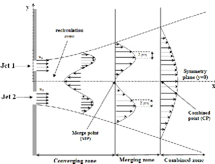
Parallel turbulent jets have numerous technological applications [1-6] such as entrainment and mixing processes in boiler and gas turbine combustion chamber, injection and carburetor systems, waste disposal plums from stacks, heating and air-conditioning systems, vertical take-off and landing of airplanes. In recent decades, this type of flow has attracted considerable interest of researchers. Several studies are available on multiple turbulent jets. The earliest studies were those of Miller and Commings [7] in which measurements of mean velocity and static pressure was carried out along the flow field of two plane parallel jets. The basic flow and entrainment mechanisms were investigated by Tanaka [8, 9] who found that the flow field consists of three relevant regions: the converging region, the merging region and the combined region. The first region, termed as the converging region, is located between the nozzle exit and the point where the two jets merge. This point is called the merge point. This region is characterized by the entrainment of the surrounding fluid by turbulent jet mixing which creates a lower pressure region wherein is formed a reverse flow. The second zone termed the merging zone, wherein the mixing between the jets occurs. This zone expands to the point where the axial velocity along the flow symmetry axis is maximum. This point is called the combined point. The last zone named the combined zone is downstream of the combined point where the two jets begin to look like a self-similar single jet. The characteristics of the flow field of the two plane parallel jets are shown in Figure 1. Murai et al. [10] experimentally studied two plane parallel jets. Measurements of pressure and stream-wise velocity were made with hot wire in the converging and combined regions while studying the effect of the nozzle converging angle.

Figure 1. Schematic diagram of two plane parallel jets

Marsters [11] carried out measurements of mean velocity and static pressure along the flow fields of two plane parallel ventilated jets. They found that the velocity profiles maintain their self-similarity behaviour only in the converging and combined regions. In addition, the distribution of the static pressure is not affected by the Reynolds number variation for

8600≤Re≤15700. Elbanna and Gahin [12]

experimentally investigated the mixing between two parallel jets. They measured the mean velocity, turbulence intensity and Reynolds shear stress. By comparing their results of two parallel jets to a single jet, they found, in the combined zone, that the dynamic half width for two jets changes linearly with the axial distance and its propagation angle is slightly smaller than that for a single jet. Elbanna and Sabbaght [13] experimentally investigated the effect of the velocity ratio on the static pressure, mean and fluctuation velocities. They found that for a velocity ratio r≠1, the weaker jet (with a low outlet velocity) is deflected towards the stronger jet (with a high outlet velocity). Lin and Sheu [14, 15] experimentally considered the nozzle spacing effect on the merge point position. Using the hot wire anemometry, Lin and Sheu [14, 15] determined the cartography of the mean velocity and Reynolds shear stress. They showed that in the converging and combined zone, the mean velocity approaches self-preservation. They also showed that the spreading rate of a two jets in the converging zone is greater than that of a single jet in the same region. Nasr and Lai [16] measured the velocity fields of two plane parallel jets. They showed that for a nozzle aspect ratio (the ratio between the length and width of the nozzle) of less than 24, the side plates should be installed to improve the two-dimensionality of the flow. In addition, they found that the flow is independent of the Reynolds number for 11000≤Re≤19300. Wang et al. [17] studied analytically the incompressible multiple jet using the Prandtl mixing length hypothesis. Their results show that in the axial direction, the axial velocity decreases as a single jet, while in the transverse direction, the velocity profile follows a cosine function whose amplitude decreases gradually with increase of the axial distance, and finally approaches a flat profile.

Spall [19] using the experimental setup of Anderson and Spall [18]. He showed that the slight change in buoyancy has a pronounced effect on the merge point location. In fact, increasing buoyancy is accompanied by a decrease in the axial merge point position, while for a Richardson number Ri>0.25, Spall [19] found that the merge point location is independent of the nozzle spacing. Suyambazhahan et al. [20] numerically studied two-plane parallel jets and compared their results to the experimental ones developed by Lin and Sheu [14] and Spall [19]. They studied the oscillation characteristics of the temperature and velocity fields. The analysiswas carried out for the Reynolds number ranging from a 9000≤Re≤12000 and at the Grashof number 50≤Gr≤1000. The comparison between the experimental measurements and the numerical ones reveal an excellent agreement in the location of the merge point and with regard to the velocity profile. They also investigated the effect of the Reynolds number, nozzle spacing and the jet inlet temperature. The mixing phenomenon in two parallel jets has numerically been studied by Durve et al. [21] using both turbulence models k  and RSM. The simulation of two jets flow is based on the experimental setup of Anderson and Spall [18]. Durve et al. [21] studied the effect of the nozzle spacing and velocity ratio on the location of the merge and combined points. They found that the location of the merge point depends not only on the nozzle spacing but also on the nozzles exit condition such as the turbulence intensity.

Through all these works we have just mentioned, it appears that the majority of studies of the two-plane parallel jets focused on determining the different zones of the flow fields and the effect of the Reynolds number, turbulence intensity and nozzle spacing on the location of the merge and the combined points. However, apart for Elbanna and Sabbagh [13] and Durve et al. [21] there has been no notable attempt to study the effect of the velocity ratio on the location of the merge and combined points. The present study complements the work of Elbanna and Sabbagh [13] and Durve et al. [21] while considering several velocity ratios.

2. MATHEMATICAL FORMULATION

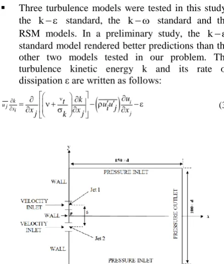
The experimental configuration of Anderson and Spall [18] is used to study the flow fields generated by the two-plane parallel turbulent jets as shown in Figure 1. Both nozzles are identical and rectangular. The width and length of each one is d=6.35mm and l=203mm, respectively. The turbulence intensity at the nozzles exit and the Reynolds number are Re=6000, I=3.6%, respectively, which relates to a velocity initial value U0=18m/s. The dimensions of the computed region are chosen so as not to affect the flow spreading. Several

configurations are tested to finally adopt the following dimensions of the computed region such as 100×d and 150×d respectively along the transverse and longitudinal directions. Figure 2 shows the dimensions adopted as well as the location of the Cartesian coordinate system. Three different spacing are used to validate our simulated numerical model including s/d=9, s/d=13 and s/d=18.25.

2. 1. Hypothesis The equations system governing the flow is written in the Cartesian coordinate system of which origin o is located in the symmetry axis of the two jets (Figure 1). The following hypothesis will also be adopted:

 The flow is steady, two-dimensional and

isothermal.

 The work fluid is air-assumed, incompressible and the thermo-physical properties are constant.

 The jet is emitted in the longitudinal direction.

 The flow is assumed to be turbulent and fully developed.

2. 2. Governing Equation The Reynolds averaged Navier-Stocks equations can be written as follows:





 _

xui_i (1)

1 

 

 

 

 

 _{ }  _  _ _{  }

   

ui p ui

u j u u_{i j}

x_j x_i x_j x_j (2)

 Three turbulence models were tested in this study: the k  _{standard, the} k  standard and the RSM models. In a preliminary study, the k  standard model rendered better predictions than the other two models tested in our problem. The turbulence kinetic energy k and its rate of dissipation ε are written as follows:

 

 

  

  

_ _ 

 



  _{ }

_  _{ }   _  

k i

u j

xi _j

u k

t _{u u}

i j

x_j x_j x

k

(3)

Figure 2. Computational region, domain size and boundary

 

2 2



 



_{ }  _{ }  _{ } 

 



   _{ } 

_  _{ }  _{  }



u j xi

j u

t _{C u u} i _C

i j

x_j x_j k x k (4)

The turbulent viscosity _t is written in terms of k and ε as follows:

2

 C k

t

 _{  } (5)

 

 

 

 

   

 _{u u}  _ui_uj

t

i j _{x x}

j i

  (6)

Solving Equations (1)-(6) requires the use of standard model constants provided by Hossain et al. [22] shown in Table 1.

2. 3. Boundary Conditions To complete the problem, besides the equations mentioned above, it is necessary to take into account the boundary conditions shown in Figure 2 and summarized in Table 2.

2. 4. Numerical Method In this work, the transport equation associated to the boundary and emission conditions are solved numerically by a finite volume method using a staggered grid. The computed region is divided into finite number of sub-regions called "control volume". The resolution method is to integrate on each control volume the transport equations such as the momentum conservation, mass conservation, the turbulence kinetic energy k and the dissipation rate of kinetic turbulence energy ε. These equations are discretized using the second order upwind. The coupling velocity-pressure is based on the SIMPLEC algorithm. A non-uniform grid is adopted in the longitudinal and transverse direction; a fine grid is used near the nozzles and a little looser further. The convergence of the global solution is obtained when the normalized residuals fall below 10-4. We have verified that the increase in this accuracy had practically no influence on the results.

3. RESULTS

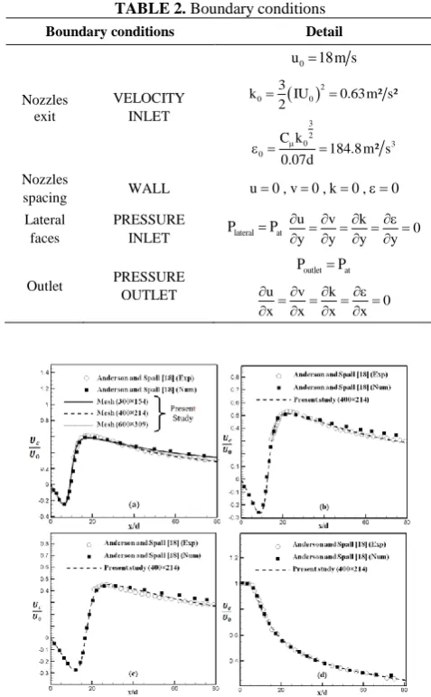
3. 1. Validation of Velocity Fields and Study of Grid Sensitivity A non-uniform grid is found adequate along the longitudinal and transverse direction; fine grids are used at the shear layers and near nozzles exit. Figure 3 shows the prediction of the axial mean velocity on the symmetry plane (y=0) using the standard

k  turbulence model for different nozzle spacing

TABLE 1. Standard model constant

Constant

1

c c2 c k 

Value 1.44 1.92 0.09 1 1.3

TABLE 2. Boundary conditions

Boundary conditions Detail

Nozzles exit

VELOCITY INLET

0

u 18m s

 2

0 0

3

k IU 0.63m² s²

2

 

3 2

0 3

0

C k

184.8 m² s 0.07d



  

Nozzles

spacing WALL u0, v0, k0, 0

Lateral faces

PRESSURE

INLET PlateralPat

u v k

0

y y y y

 _ _ __

   

Outlet PRESSURE

OUTLET

outlet at

P P

u v k

0

x x x x

 _ _ __

   

Figure 3. Axial velocity distribution along the symmetry axis.

(a) s/d=9, (b) s/d=13, (c) s/d=18.25,(d) Single jet

Figure (3d) shows the prediction of the axial mean velocity for the single jet flow along the symmetry axis using the k  standard turbulence model. An analysis of this figure shows a very good agreement with the experimental results of Anderson and Spall [18] for the single jet case.

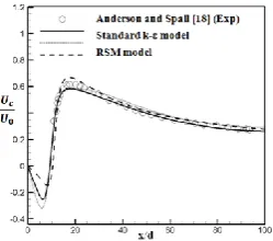
In Figure 4, we report the x=0) for a nozzle spacing s/d=9 using three turbulence models: k  standard, k  standard and RSM. Note that the k standard shows better agreement with the experimental results of Anderson and Spall [18] in the converging and combined zones. However, a slight difference is observed in the merge zone while the other two models over-predict the axial velocity in the merge and combined zones.

3. 2. Nozzle Spacing and Velocity Ratio Effect Figures (5a) and (5b) show the axial location, respectively, of the merge and combined points with respect to the nozzle spacing s/d for a velocity ratio r=1, alongside the results of the previous investigation. This figure shows that the merge and combined points axial location increase with the nozzle spacing. For r=1, the merge and combined points always keep their locations on the symmetry axis (y=0). This increase in the axial location is linear for the nozzle spacing ranging 6≤s/d≤39 and can be represented by the following formulas:

 

1.01 0.4

mp

x d  s d  (7)

 

0.895 9.66

cp

x d  s d  (8)

From this figure (Figure 5), we can note that our results are in good agreement with some previous results (Anderson and Spall [18], Militzer [23] and Miller and Commings [7]) and different from some others (Lin and Sheu [14], Tanaka [9] and Murai et al. [10]). Indeed, the jet exit conditions adopted in each study are not completely identical. Thus, the merge and combined point location greatly depend on the nozzles exit conditions such as the nozzle spacing s, jet exit velocityU₀, turbulence intensity I₀ and the geometry of the nozzle, etc.

Figures (6a) and (6b) show respectively the variation of the axial xmp d _{and the transverse} ymp d location of merge point with respect to the spacing between the nozzles and for different velocity ratios. For a fixed spacing, the axial location of the merge point decreases for a high velocity ratio (Figure (6a)), while its transverse location increases with the velocity ratio (Figure (6b)). Figure 6 also shows that for r=1 and for different nozzle spacing, the merge point occurs always on the symmetry axis (y=0) as established by Anderson and Spall [18], Lin and Sheu [14], Tanaka [9], Militzer

Figure 4. Sensitivity of center line velocity profile to turbulence models

Figure 5. Variation in axial location of merge and combined point (a) Merge point, (b) Combined point

Figure 6. Variation in merge point location: (a) Axial

location, (b) Transverse location

Consequently, the nozzle spacing effect on the axial position of the merge point is less remarkable for a velocity ratio r>1 (Durve et al. [21]). This can be explained by the fact that the transverse velocity magnitude for r>1 is greater than that for r=1. The axial and transverse locations of the merge point shown in Figure 6 are sensitive to the velocity ratio and the nozzle spacing. Therefore, these different parameters are

correlated by the following equations:

 

1.517 

  

mp

x d r s d (9)

 

0.024

  

mp

y d r s d (10)

These correlations predict the axial and transverse positions of the merge point respectively, with an average error of 2.6% and 9.7%. In addition, the velocity ratio and the spacing between the nozzles strongly affect the combined point location. In Figure 7, we show the effect of velocity ratio and nozzle spacing on the axial and transverse location of combined point. This figure shows that for a fixed nozzle spacing, the axial position of the combined point moves further upstream when the velocity ratio increases while its transverse location increases with the velocity ratio. We note then, that increasing the velocity ratio promotes the appearance of the combined point upstream. The changes in the combined point positions are linear which allows us to propose the correlations below connecting the combined point position with the

velocity ratio and nozzle spacing.





6.379 

  

cp

x

r s d

d (11)





0.168

  

cp

y

r s d

d (12)

These correlations predict the axial and transverse positions of the combined point respectively, with an average error of 2.2% and 3%.

Equations (9) and (11) predict the merge and combined points longitudinal positions for 6 S 13 and 1 r 2 while Equations (10) and (12) predict the merge and combined points transverse positions for 6 S 13 and 1.2 r 2, since for r=1 the merge and combined points are located on the symmetry axis





3. 3. Jet Spreading The jet spreading can be judged by examining the two criteria: the maximum centerline velocity U_m decay and the growth of the half widthy_0.5.

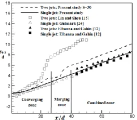
3. 3. 1. Maximum Velocity Decay (r=1) The longitudinal distribution of the maximum centerline velocity U_m is represented in Figure 8 for the three

Figure 7. Variation in combined point location. (a) Axial location, (b) Transverse location

Figure 8. Maximum velocity decay for different zone

zones of the two jets flow: the converging zone, merging zone and the combined zone for a nozzle spacing s/d=30. Note that the maximum velocity decreases hyperbolically depending on the axial positions in the converging and the combined zone while, in the merging zone, it is too difficult to describe

m

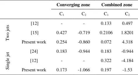
U curve with a meaningful function. In both zones (converging and combined zone), numerical solutions can be approximated by a function which can be written as follows:

 2  

0 m  1  2

U U C x d C (13)

case, is also raised by Lin and Sheu [15] who found that 1

C 0 427. is greater than the value C10 183. established by Gutmark [24] for the single jet. In the combined zone, this coefficient for the two jets, is equal to 0.072, which is lower than that for the single jet (0.197). Consequently, in the combined zone, the spreading of two jets is lower than that for the single jet. This observation is in good agreement with that reported by Elbanna and Gahin [12], C₁0 133. which is lower than that for the single jet





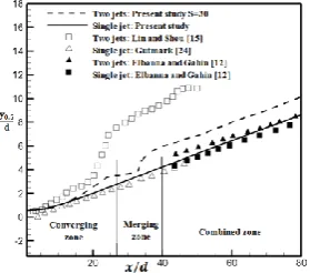
3. 3. 2. Dynamic Half Width Evolution (r=1) Figure 9 shows that the axial distribution of the dynamic half-width

y

TABLE 3. Coefficients of linear function in two different zones

TABLE 4. Jet exit conditions and nozzle dimensions

Experiment U0(m/s) d (mm) I (%)

[24] 35 13 0.2

[12] 24 12 1

[15] 57 2 0.8

[18] 18 6.35 3.6

TABLE 5. Coefficients of linear function in two different zones

Converging zone Combined zone

K1 K2 K1 K2

Tw

o

j

et

s [12] - - 0.092 1.240

[15] 0.1828 -0.0078 0.1553 0.1174

Present work 0.146 -0.471 0.105 1.680

S

in

g

le

j

et [24] 0.1015 -0.1101 0.1015 -0.1101

[12] - - 0.101 -0.035

Present work 0.110 -0.147 0.110 -0.147

We notice that y_{0 5}. increases linearly in the convergence

and combined zones according to the following expression:





0 5.  1  2

y d K x d K (14)

1

K is the expansion coefficient of the dynamic half-width and K₂is the virtual origin. The values of these coefficients are given in Table 5. The observations for the maximum velocity decay are reinforced by a quick analysis of values in Table 5 which allows us to deduce that in the converging zone, a better two jets spreading may occur in compare to single jet. A good agreement is noted with the results of Lin and Sheu [15] for two jets and of Gutmark [24] for the single jet in the converging zone, while in the combined zone, the two jets spreading is less than that for the single jet (Elbanna and Gahin [12]).

3. 4. Jet Spreading in the Converging Zone For a velocity ratio r=1, the jet spreading is the same in the halves planes y/d>0 and y/d<0 (Figure 1). Indeed, the flow field has a symmetry axis defined as y=0. The increasing of the velocity ratio is performed by decreasing the initial velocity of the jet contained in the half plane y/d<0, while keeping constant the initial jet velocity contained in the half plane y/d>0. Consequently, for r>1, the y/d>0 zone became the one which contains the strongest jet (jet 1), and the y/d<0 zone becomes the one which contains the weakest jet (jet 2) (Figure 1). In the following section, our work is focused on studying the velocity ratio effect on the stronger and lower jet spreading in the converging zone.

3. 4. 1. Strong Jet Figures (10a) and (10b) show the longitudinal distribution of the maximum velocity U_m on the strong jet axis and the growth of the strong jet dynamic half-width y0.5 for different velocity ratios. The maximum velocity and the dynamic half-width are respectively normalized by the maximum axial velocity and the half width of the strong jet at distance of x/d=1, since x/d=1 lies within the potential core region for both the strong and weak jets for different velocity ratios. The results show that in the vicinity of the nozzle exit, the maximum velocity (Figure (10a)) and the dynamic half-width of the strong jet (Figure (10b)) are constant and equal to their values at the jet exit for different velocity ratio. Further, the maximum velocity decay and the dynamic half-width growth of the strong jet decrease as the velocity ratio increases. This behavior corresponds to a slower strong jet spreading for a greater velocity ratio. In fact, the increase of the velocity ratio is accompanied by a decrease in the low jet initial velocity while keeping constant the strong jet initial velocity.

Converging zone Combined zone

C1 C2 C1 C2

Tw

o

j

et

s [12] - - 0.133 0.497

[15] 0.427 -0.719 0.2106 1.8201

Present work 0.254 -0.860 0.072 4.318

S

in

g

le

j

et [24] 0.183 -0.944 0.183 -0.944

[12] - - 0.322 -4.184

Figure 9. Dynamic half width for different zone

Figure 10. Maximum velocity decay and half width for strong

jet. (a) Maximum velocity decay, (b) Half width

Figure 11. Maximum velocity decay and half width for weak

jet. (a) Maximum velocity decay, (b) Half width

Figure 12. Velocity ratio effect on maximum velocity decay and jet half width, (a) Maximum velocity decay, (b) Half width

Hence, the weak jet produces some braking on the strong jet, which decelerates its spread.

3. 4. 2. Weak Jet Figure 11 shows the longitudinal evolution of the maximum velocity on the weak jet axis (Figure (11a)) and the dynamic half-width of the weak

jet (Figure (11b)). The maximum velocity and the dynamic half-width are respectively normalized by the maximum axial velocity and the dynamic half-width of the weak jet at the distance x/d=1. The analysis of this figure shows that the velocity profiles as well as the dynamic half-width are identical in the vicinity of the nozzles exit. Further, the maximum velocity decay (Figure (11a)) and the weak jet spread (Figure (11b)) increase with the velocity ratio due to the strong jet dominance. Indeed, the weak jet is attracted by the strong jet, so the strong jet produces some acceleration on the weak jet which enhances its spread. From Figures (10a) and (11a), we see that the maximum velocity evolution of the strong jet and the weak jet decreases hyperbolically with the longitudinal distance x d according to Equation (13). The decay coefficients of the maximum velocity C1 for the strong and weak jets, determined by a numerical simulation, are shown in Figure (12a) for different velocity ratios. The results show that the coefficient C1 of the strong jet decreases as the velocity ratio increases, while for the weak jet, the coefficient C1 increases with the velocity ratio. Figures (10b) and (11b) show that the dynamic half-width of the strong and weak jet increases linearly with

x d according to Equation (14). The dynamic half-width expansion coefficients K1 of the strong and weak jet are plotted in Figure (12b) for different velocity ratios. The results show that when the velocity ratio increases, the dynamic half-width expansion coefficient K1 of the strong jet decreases while that of the weak jet increases, which is in coherence with the velocity decay behavior. Indeed, the weak jet expansion increases and decreases for the strong jet. This is evident because the weak jet will be attracted by the strong jet, which accelerates its expansion.

4. CONCLUSION

nozzle spacing effect on the axial location of the merge and combined point decreases by increasing the velocity ratio while this effect on the transverse positions increase. The axial and transverse positions of the merge and combine points evolution according to the velocity ratio r and the nozzle spacing s is described by Equations (9)-(12). The increase in the velocity ratio results that the weak jet exercises some braking on the strong jet, which decelerates its spread. On the other hand, the increase in the velocity ratio results that the strong jet produces some acceleration on the weak jet, which enhance its spread.

5. REFERENCES

1. Ahmed, S., Ali, M. and Sadrul Islam, A., "A numerical study on mixing of transverse injection in supersonic combustor",

International Journal of Engineering-Transactions A: Basics,

Vol. 17, No. 1, (2003), 85-93.

2. Hematian, J., "Appropriate loading techniques in finite element analysis of underground structures", International Journal of

Engineering, Vol. 11, No. 1, (1998), 43-52.

3. Kahrom, M., Farievar, S. and Haidarie, A., "The effect of square splittered and unsplittered rods in flat plate heat transfer enhancement", International Journal of Engineering, Vol. 20, No. 1, (2007), 83-94.

4. Shamsi, M. and Nassab, S. G., "Ivestigation of entropy generation in 3-D laminar forced convection flow over a backward facing step with bleeding", International Journal of

Engineering-Transactions A: Basics, Vol. 25, No. 4, (2012),

379-388.

5. Abbasalizadeh, M., Jafarmadar, S. and Shirvani, H., "The effects of pressure difference in nozzle’s two phase flow on the quality of exhaust mixture", International Journal of

Engineering-Transactions B: Applications, Vol. 26, No. 5, (2013), 553-562.

6. Sikarwar, B., Bhadauria, A. and Ranjan, P., "Towards an analytical model for film cooling prediction using integral

turbulent boundary layer", International Journal of

Engineering-TransactionsA: Basics, Vol. 29, No. 4, (2016),

554-562.

7. Miller, D. R. and Comings, E. W., "Force-momentum fields in a dual-jet flow", Journal of Fluid Mechanics, Vol. 7, No. 02, (1960), 237-256.

8. Tanaka, E., "The interference of two-dimensional parallel jets: 1st report, experiments on dual jet", Bulletin of JSME, Vol.

13, No. 56, (1970), 272-280.

9. Tanaka, E., "The interference of two-dimensional parallel jets: 2nd report, experiments on the combined flow of dual jet",

Bulletin of JSME, Vol. 17, No. 109, (1974), 920-927.

10. Mural, K., Taga, M. and Akagawa, K., "An experimental study on confluence of two two-dimensional jets", Bulletin of JSME, Vol. 19, No. 134, (1976), 958-964.

11. Marsters, G., "Interaction of two plane, parallel jets", AIAA

Journal, Vol. 15, No. 12, (1977), 1756-1762.

12. Elbanna, H., Gahin, S. and Rashed, M., "Investigation of two plane parallel jets", AIAA Journal, Vol. 21, No. 7, (1983), 986-991.

13. Elbanna, H. and Sabbagh, J., "Interaction of two non-equal plane jets", AIAA Journal, Vol. 25, (1985), 12-13.

14. Lin, Y. and Sheu, M., "Investigation of two plane paralleltiinven ilated jets", Experiments in Fluids, Vol. 10, No. 1, (1990), 17-22.

15. Lin, Y. and Sheu, M., "Interaction of parallel turbulent plane jets", AIAA Journal, Vol. 29, No. 9, (1991), 1372-1373. 16. Nasr, A. and Lai, J., "Two parallel plane jets: Mean flow and

effects of acoustic excitation", Experiments in Fluids, Vol. 22, No. 3, (1997), 251-260.

17. Wang, J., Priestman, G. H. and Wu, D., "An analytical solution for incompressible flow through parallel multiple jets", Journal

of Fluids Engineering, Vol. 123, No. 2, (2001), 407-410.

18. Anderson, E. A. and Spall, R. E., "Experimental and numerical investigation of two-dimensional parallel jets", Journal of

Fluids Engineering, Vol. 123, No. 2, (2001), 401-406.

19. Spall, R. E., "A numerical study of buoyant plane parallel jets", Transactions-American Society of Mechanical Engineers

Journal of Heat Transfer, Vol. 124, No. 6, (2002), 1210-1212.

20. Suyambazhahan, S., Das, S. K. and Sundararajan, T., "Numerical study of flow and thermal oscillations in buoyant twin jets", International Communications in Heat and Mass

Transfer, Vol. 34, No. 2, (2007), 248-258.

21. Durve, A., Patwardhan, A. W., Banarjee, I., Padmakumar, G. and Vaidyanathan, G., "Numerical investigation of mixing in parallel jets", Nuclear Engineering and Design, Vol. 242, (2012), 78-90.

22. Hassain, M. and Rodi, W., "A turbulence model for buoyant flows and its application to vertical buoyant jet", Turbulent Jets

and Plumes, Pergamon Press, Oxford, (1982), 121-178.

23. Militzer, J., "Dual plane parallel turbulent jets", University of Waterloo, Ph.D. Thesis, (1977).

24. Gutmark, E. and Wygnanski, I., "The planar turbulent jet",

Numerical Study of Interaction of Two Plane Parallel Jets

N. Hnaiena_{, S. Marzouk Khairallah}a_{, H. Ben Aissia}a_{, J. Jay}b

a _{Unite of Metrology and Energy Systems, National Engineering School of Monastir, Monastir, Tunisia}

b _{Thermal Center of Lyon, INSA Lyon, France}

P A P E R I N F O

Paper history: Received 26 July 2015

Received in revised form 05 August 2016 Accepted 30 August 2016

Keywords: Combined Point Merge Point Spacing Turbulent Two Jets Velocity Ratio هديكچ رد صٍّژپ ،رضاح ی ک ثض ی ِ زاس ی ددع ی ٍد تج ِتفضآ حطسه زاَه ی ِئارا ُدض تسا . دٌچ ی ي لده گتفضآ ی رد راک رضاح درَه اهزآ ی ص رارق ،دٌتفرگ زا ِلوج :

k 

،درادًاتسا

k 