A Low Cost Numerical Simulation of a Supersonic Wind-tunnel Design

Please cite this article as: H. Bagheri-Esfe, M. Dehghan Manshadi, A Low Cost Numerical Simulation of a Supersonic Wind-tunnel Design, International Journal of Engineering (IJE), IJE TRANSACTIONS A: Basics Vol. 31, No. 1, (January 2018) 128-135

International Journal of Engineering

A Low Cost Numerical Simulation of a Supersonic Wind-tunnel Design

H. Bagheri-Esfea_{, M. Dehghan Manshadi}*b

a _{Faculty of Engineering, University of Shahreza, Shahreza, Iran}

b _{Department of Mechanical & Aerospace Engineering, Malek-Ashtar University of Technology, Isfahan, Iran} P A P E R I N F O

Paper history: Received 17 July 2017

Received in revised form 26 November 2017 Accepted 30 November 2017

Keywords: Geometrical Design OpenMp Recovery Factor Roe Scheme

Supersonic Wind-Tunnel

A B S T R A C T

In the present paper, a supersonic wind-tunnel is designed to maintain a flow with Mach number of 3 in a 30cm×30cm test section. An in-house CFD code is developed using the Roe scheme to simulate flow-field and detect location of normal shock in the supersonic wind-tunnel. In the Roe scheme, flow conditions at inner and outer sides of cell faces are determined using an upwind biased algorithm. The in-house CFD code has been parallelized using OpenMp to reduce the computational time. Also, an appropriate equation is derived to predict the optimum number of cores for running the program with different grid sizes. In the design process of the wind-tunnel, firstly geometry of the nozzle is specified by the method of characteristics. The flow in the nozzle and test section is simulated in the next step. Then, design parameters of the diffuser (convergence and divergence angles, area of the throat, and ratio of the exit area to the throat area) are determined by a trial and error method. Finally, an appropriate geometry is selected for the diffuser which satisfies all necessary criteria.

doi: 10.5829/ije.2018.31.01a.18

1. INTRODUCTION1

Wind-tunnel is a tool used in aerodynamic research to study effects of the air moving over solid objects. The earliest enclosed wind-tunnel was invented in 1871 by Francis Herbert Wenham. The Wright brothers' use of a simple wind-tunnel in 1901 to study effects of airflow over various shapes was in some ways revolutionary [1]. Then, Blair et al. [2] designed a large-scale wind- tunnel for simulation of turbomachinery airfoil boundary layers. Lacey [3] reviewed new developments

*Corresponding Author’s Email: [email protected] (M. Dehghan Manshadi)

in automotive wind-tunnels. Afterwards, Potts et al. [4] developed a transonic wind-tunnel test bed for MEMS flow control. Dehghan Manshadi et al. [5] proposed a two-level scheme involves Schlieren image processing and classification to detect normal shocks in wind-tunnels.

In addition to experimental investigations, some numerical studies have been performed in the design and simulation of wind-tunnels. For example, Thibodeaux and Balakrishna [6] developed a hybrid-computer simulator for a transonic wind-tunnel. Szuch et al. [7] presented dynamic simulations of a subsonic wind-tunnel. Afterwards, Shono et al. [8] designed a NOMENCLATURE

AF Area factor nt Number of threads

Et Total internal energy (Nm) Q Conservative vector

F Parallel fraction of the code S Local speedup

RF Recovery factor T Temperature (K)

F1inv Horizontal inviscid flux vector u,v Velocity components (m/s)

G1inv Vertical inviscid flux vector Greek Symbols

Ht Total enthalpy (Nm)  Density (kg/m3)

J Jacobian  Limiter function

virtual two-dimensional wind-tunnel using a vortex element method. Kouhi et al. [9] performed geometry optimization of the diffuser for the supersonic wind-tunnel using genetic algorithm. Then, M. Rabbani et al. [10] carried out a numerical simulation using finite volume method to investigate behavior of transient shock wave and effect of various stagnation temperatures on the features of flow-field in the blowdown supersonic wind-tunnel.

According to the literature review, different numerical methods have been used to simulate flow-field in the wind-tunnels. In this paper a supersonic wind-tunnel is designed using Roe scheme. Roe scheme is a robust, high resolution and non-oscillatory method to simulate compressible flows [11, 12].

Due to large number of iterations required for design of a wind-tunnel, the CPU time for every iteration of the program is very important. One of the most effective methods to reduce this time is parallel processing.

Parallel processing has wide applications to solve time-consuming problems. For example, Rajan [13] developed an algorithm for subsonic compressible flow over a circular cylinder. Afterwards, Barth et al. [14] used a parallel non-overlapping domain-decomposition algorithm for compressible fluid flow problems on triangulated domains. Aliabadi [15] reported the performance of a parallel implicit finite volume solver for compressible flows. Koobus at al. [16] presented parallel simulations of three-dimensional complex flows on homogeneous and heterogeneous computational grids. Then, He et al. [17] used MPI to develop parallel simulation of compressible fluid dynamics using lattice Boltzmann method. In 2013, Xu et al. [18] used MPI+OpenMP hybrid parallel algorithm to optimize numerical simulation of two-dimension compressible flow-field in the multi-core CPU cluster parallel environment.

As pointed out earlier, numerical simulation of flow-field in the wind-tunnel is very time-consuming. Thus, in this paper a parallel algorithm has been developed using OpenMp to reduce computational time of the program. Also, an appropriate equation is derived to predict the optimum number of cores for running the program with different grid sizes. This is the main novelty of this paper.

2. GOVERNING EQUATIONS

The governing equations for the inviscid, unsteady and compressible flow in full conservative form are written as [19]:

(1)

where Q1 is the vector of conservative variables and

F1inv, G1inv are inviscid flux vectors in  and directions, respectively. The conservative variables and inviscid flux vectors in generalized coordinates are connected to those in physical space using:

(2)

where xyxyare metrics and J is the Jacobian of

transformation. Also:

(3)

where  is density, P is static pressure and u, v are horizontal and vertical velocity components, respectively. Et is total energy and Ht is total enthalpy.

3. NUMERICAL DISCRETIZATION

3. 1. Temporal Discretization Using a forward Euler scheme for the time derivative, Equation (1) is written in a semi-discrete form as:

(4)

where superscript n represents the iteration number. The value of Q1n+1 is determined from Equation (4), so all the primitive variables at the new time step (n+1) are obtained [20].

3. 2. Spatial Discretization In the Roe scheme,

the inner and outer flow conditions are determined using either the first, second, or third-order upwind biased algorithm. Extrapolation of the primitive variables such as pressure, velocity and temperature from the cell centers to the cell faces, is performed by the MUSCL strategy [21]. To determine the variables at the east face of the control volume (E), the following relations are used:

(5)

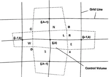
where L and R denote the left and right sides of each cell face, respectively, as shown in Figure 1.

1 1inv 1inv ₀

Q F G

t  

  

  

  

1

1

1

,

,

y x inv

y x inv

Q Q

J

F F G

J J

G F G

J J

 

 



 

 

2

2

, ,

t t t

u v

uv

u P u

Q F G

v uv P v

E uH vH

 





 

  

  

   

 

   

  _

   

 

 _{ } _{ }

  

   

 

   

     

1

1 1 ₍ 1 _{) (} 1 _{) 0}

n n

n n

inv inv

Q Q F G

t  

 _{  }

  

  

,

1, 1

(1 ) (1 )

4 1

(1 ) (1 )

4

L

E i j W E

R

E i j EE E

q q q q

q q q q

 

 



  _      _

Figure 1. Arbitrary configuration of grid lines with the corresponding cell-vertex control volume allocated to each node

In Equation (5), q represents any of the four primitive variables, i.e q





1, ,

,_Eqq_{i j}q_{i j} and _EEqq_i2,jq_i1,j. Also, =-1 and =1/3 correspond, respectively, to the second order upwind and the third order upwind-biased algorithms. For the first order algorithm, the L and R side values of the primitive variables at the east face, are determined

from L _,

E i j

q q and R _1,

E i j

q q . A similar formula can be

written for the inner (L) and outer (R) values at the north face of the control volume.

The van Albada flux limiter is used for damping the spurious numerical oscillation in high resolution computations, written as [22]:

(6)

The limiter function  is defined by:

(7)

where ε is a small value for preventing indeterminate value in regions of uniform flow, where the values of

Wq

 and Eqare near zero.

An entropy correction method is used to avoid expansion shocks in the regions where the eigenvalues become equal to zero. The relevant equation is written as:

(8)

where Land Rare the eigenvalues determined at the inner and outer flow conditions, respectively. Also, ˆ is

the eigenvalue of the Jacobian matrix of the flux vector determined at Roe’s averaged condition [19].

3. 3. Roe’s Numerical Flux Scheme The inviscid

flux vectors using the Roe scheme is obtained from the following formulae:

(9)

(10)

Here,  is the eigenvalue of the Jacobian matrix, T the corresponding eigenvector and w the wave amplitude vector. More details of Equations (9) and (10) can be found in [11].

3. 4. Roe’s Averaging The square root of density at

the left (L) and right (R) sides of east face of a cell, are called weighting factors. These variables ( L, R)

E E

W W are

determined as follows:

(11)

The numerical flux for the Roe scheme is calculated at the so-called Roe-averaged values, which are obtained from the inner L and outer R state values at the sides of east (E) cell face asfollows:

(12)

(13)

(14)

Similar formulas can be written for the quantities on the north side of a cell face [12].

3. 5. Validation of the Developed CFD Code To

validate the Roe scheme in the CFD code, numerical results are compared with the experimental data of Emery et al. [23] for flow over NACA 65-410 blade. In Figure 2, pressure coefficient (Cp) on the surface of

NACA 65-410 blade is plotted. As observed in this figure, the numerical results are in good agreement with the experimental data of Emery et al. [23].

,

1,

(1 ) (1 )

4

(1 ) (1 )

4

L

E i j W E

R

E i j EE E

q q q q

q q q q

 _{ }

 _{ }



  _      _

  _      _

, _{2 2}

2( )( )

( ) ( ) W E i j W E q q q q           



 



ˆ ˆ _{2 if}

ˆ ˆ

4 max 0, ,

new L R                  _   _   4 ( ) ( ) ( ) 1

1 1 _{ˆ ˆ}

( )

2 2

L R k k k

E E E E E E

k

F F F  w T



  



4

( ) ( ) ( )

1

1 1 _{ˆ ˆ}

( )

2 2

L R k k k

N N N N N N

k

G G G  w T



  



,

L L R R

E E E E

W   W  

ˆ_E W W_EL. _ER

 

ˆ ,

ˆ

L L R R

E E E E

E _{L R}

E E

L L R R

E E E E

E _{L R}

E E

W u W u

u

W W

W v W v

v W W      

ˆ EL EL ER ER

E L R

E E

W H W H

H

W W

 

x/c

Numerical Result Experimental Data [24]

Figure 2. Comparison between numerical results using the Roe scheme and experimental data of Emery et al. [24]; Distribution of pressure coefficient (Cp) on the NACA 65-410

blade

4. PARALLEL ALGORITHM

As pointed earlier a trial and error method is used to design the wind-tunnel in this paper, so the numerical program should be iterated several times. To speed up the computations, a multiprocessor computer has been used. In order to utilize the computing resources, a parallel code has been developed using OpenMp. In this section, parallelization strategy of the program is described and performance of the parallel program is studied.

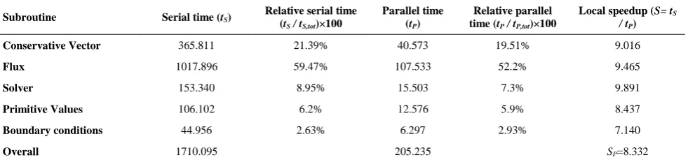
4. 1. Parallelization Strategy Table 1 shows the

computational time of different subroutines related to serial and parallel programs. For the parallel program, the number of nodes (N) and threads (nt) are equal to

27000 and 10, respectively.

TABLE 1. Computational time of different subroutines related to serial and parallel programs

Subroutine Serial time (tS) Relative serial time _(t

S / tS,tot)×100

Parallel time (tP)

Relative parallel time (tP / tP,tot)×100

Local speedup (S= tS

/ tP)

Conservative Vector 365.811 21.39% 40.573 19.51% 9.016

Flux 1017.896 59.47% 107.533 52.2% 9.465

Solver 153.340 8.95% 15.503 7.3% 9.891

Primitive Values 106.102 6.2% 12.576 5.9% 8.437

Boundary conditions 44.956 2.63% 6.297 2.93% 7.140

Overall 1710.095 205.235 SP=8.332

As observed in Table 1, parallelization of subroutines can accelerate process of the program. A parallel region is built during repetition loop of the program. Threads are generated at the start of every iteration, but work sharing is done inside each subroutine. More details about method of OpenMp are explained in [24, 25].

4. 2. Analysis of the Parallel Performance Table

1 shows the value of speedup (S=tS/tP) for different

subroutines, where tS and tP are execution time for serial

and parallel codes, respectively. Also, as observed in Table 1, speedup gain in the parallel section (SP) is 8.33.

Speedup (S) is a prominent factor for estimation of performance gained by parallelization. This parameter is defined using the Amdahl’s law as follows:

(15)

where F is fraction of code that has been parallelized and SP is speedup gain in the parallel section. Parallel

section speedup (SP) is a function of number of threads

(nt) and number of nodes (N). Dependency of SP to nt

and N can be shown by the following equation: (16)

in which the coefficient  depends on N and is independent of nt.

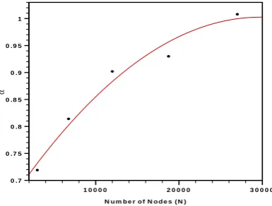
Table 2 shows values of F and  for different number of nodes. As observed in this table, parallel fraction of the code (F) is practically constant.

TABLE 2. Values of F and  for different number of nodes (N)

N F 

3000 0.988 0.719

6750 0.988 0.814

12000 0.986 0.902

18750 0.988 0.930

27000 0.987 1.008

1

(1 )

P

S

F F

S



 

( )

P t

Values of  for different grid sizes are plotted in Figure 3. A quadratic curve is fitted to these data with the following equation:

(17)

Speedup of the code for finer grids (N>27000) is estimated using Equations (15)-(17) as follows:

(18)

Amount of speedup versus number of threads for different number of nodes is plotted in Figure 4. For the case N=27000, values obtained from Equation (18) (solid line) are compared with the measured data. As observed in Figure 4, results of the Amdahl’s law are in a good agreement with the measured data for N=27000. Now, optimum number of cores for running the program with a specific grid size can be determined.

Figure 3. Variations of  with number of nodes (N)

Figure 4. Amount of speedup versus number of threads for different number of nodes (N)

Optimum number of threads for a program is determined using the condition dSn optimumt, E, where E

is a constant parameter indicating speedup variation and is considered equal to 10% in the current study. In fact, by using the optimum value of nt, there is limited

variations of speedup equal to E. The limiting condition

,

( )

t

n optimum

dS E is simplified using the following equation:

(19)

As we know dnt1. Thus:

(20)

The optimum number of cores for a program is determined using Equations (18) and (20) as follows:

(21)

The optimum value of ntfor different number of nodes

(N) is plotted in Figure 5. As shown in this figure, optimum value of ntincreases with number of nodes.

Because increase of N results increase of grid size and computational time. Thus nt and nt,opt increase with N.

5. DESIGN OF THE WIND-TUNNEL

In this section, a complete model of the wind-tunnel is designed. Different parts of the wind-tunnel (nozzle, test section, diffuser) are studied and the best geometry is selected based on the design parameters. The general schematic of the wind-tunnel is shown in Figure 6.

Figure 5. Optimum value of threads (nt,opt) for different

number of nodes (N)

10 2 5

( )N 3.778 10 N 2.25 10 N 0.6676

 _{  }  _{ }  _

10 2 5

1

(1 )

0.987

( 3.778 10 2.25 10 0.6676)

t

t

S

F F

n

N N n



 

 

 

     

N u m b e r o f N o d e s ( N )



1 0 0 0 0 2 0 0 0 0 3 0 0 0 0 0 .7

0 .7 5 0 .8 0 .8 5 0 .9 0 .9 5 1

t t

S

dS dn

n



 



,

t

n optimum t

S

dS E

n



 



10 2 5

0.985

( ) 0.985 0.015 ,

3.778 10 2.25 10 0.6676

t optimum

n

E

N N

 _

  

 

_  _

 

Figure 6. General schematic of the wind-tunnel

Geometry of the nozzle is designed using the method of characteristics. The present wind-tunnel is designed to maintain flow with Mach=3 in a 30cm×30cm test section. Then, the flow passing through the nozzle and test section is simulated and length of the test section is determined by a trial and error method. In the next step, design variables of the diffuser (length and height of the throat, convergence and divergence angles and ratio of the exit area to the throat area) should be determined.

An appropriate indicator to study performance of the wind-tunnel is defined as follows:

0 e

0

( ) ( )i

P RF

P

 (22)

where RF, (P0)e and (P0)i are recovery factor, outlet

pressure of the diffuser and inlet pressure of the nozzle, respectively. The wind-tunnel should be designed with the maximum value of recovery factor. Also, geometry of the diffuser should be designed so that a normal shock occurs at the divergent section of the diffuser close to the throat. This shock turns the outlet flow of the wind-tunnel to subsonic and increases the static pressure. These are the criteria which considered in the design process of the wind-tunnel.

5. 1. Design of the Supersonic Nozzle As pointed out earlier, the value of Mach number at the exit section of the nozzle should be equal to 3. The supersonic nozzle has been designed using the method of characteristics. In the next step of the design process, flow passing through the nozzle and test section is simulated. Length of the test section is determined equal to 1.5D (D is the test section height, D=30cm) by the trial and error method.

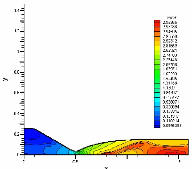
Figure 7 shows Mach number contours in the nozzle and test section. As observed in this figure, Mach number is almost equal to 3 in the test section. The grid size of the nozzle and test section is determined 144×50 after grid independency test.

5. 2. Design of the diffuser Diffuser retrieves the static pressure in the wind-tunnel. As pointed out earlier, design parameters of the diffuser are convergence and divergence angles, length and height of its throat and ratio of outlet area to throat area (area factor). Each parameter is determined using the trial and error method.

Figure 7. Mach number contours in the nozzle and test section

The optimum diffuser has minimum value of stagnation pressure loss and recovery factor (RF). Also, the appropriate wind-tunnel should pass the start condition successfully and reach to the steady state condition.

In the start condition, the inlet stagnation pressure of the nozzle is equal to 612418 pa. In the steady state condition, this value reduces to 233303pa after transition time (ttr=0.18s). In fact, after this time the

wind-tunnel reaches to the steady state condition. In this condition the Mach number in the test section equals 3 and a normal shock is formed in the divergent section of the diffuser. This shock turns the outlet flow of the tunnel to subsonic. Appropriate cross area for position of the normal shock is equal to 1.1 At, which At is area

of the diffuser throat. At this position, the normal shock has the best stability condition [26]. Thus recovery factor and position of the normal shock are two important factors to design the diffuser.

Design parameters of the diffuser are determined by the trial and error method. Different geometries should be tested and the best one selected so that the previous criteria satisfied. Convergence and divergence angles of the diffuser are selected as 30 and 3 degrees, respectively. Also, length and height of throat of the diffuser are determined equal to 5D and 0.7D, respectively, where D is the height of the test section (30cm).

The final design parameter of the diffuser is area factor ( e)

t

A AF

A

TABLE 3. Values of recovery factor (RF) and normal shock position for different geometries of diffuser

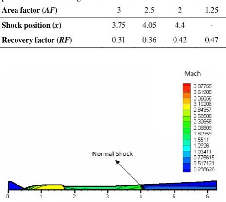
Area factor (AF) 3 2.5 2 1.25 Shock position (x) 3.75 4.05 4.4 - Recovery factor (RF) 0.31 0.36 0.42 0.47

Figure 8. Mach number contours for the case AF=2.5

Table 3 shows that recovery factor increases with area factor reduction. Also, as observed in Figure 8 and Table 3, the normal shock moves towards the outlet section of the diffuser when the area factor decreases. Also, the value of static pressure increases across the normal shock in the diffuser. Reduction of area factor (AF) decreases diffuser length. Thus, formation of the normal shock is postponed until the static pressure reaches to outlet pressure in the exit section of the diffuser.

When AF becomes 3 or 2.5, position of the normal shock is more suitable than other cases. Because it occurs at a place with area almost equal to 1.1At, thus

the shock has better stability in comparison to other cases. The best value for area factor of the diffuser is 2.5. Because the normal shock is close to the throat and its recovery factor is more appropriate than the case

AF=3.

6. CONCLUSION

Different parts of a supersonic wind-tunnel (nozzle, test section and diffuser) were designed in this paper using the Roe scheme. Suitable geometries for these parts were designed with the following criteria: Firstly, to have an almost uniform flow with Mach=3 at the test section. Secondly, to form a normal shock at the divergent part of the diffuser, close to its throat. This shock turns the outlet flow of the wind-tunnel to subsonic. Thirdly, to have a low value of stagnation pressure loss and recovery factor (RF). In the design process, in the first step, the nozzle was designed using the method of characteristics so that it can provide the

flow with Mach=3 at the nozzle outlet. Then, appropriate geometries for the test section and diffuser were selected. To reduce the computational time, a parallel program was developed using OpenMp. Also, an appropriate equation was derived to predict the optimum number of cores for a program with different grid sizes. The most important conclusions of this paper are as follows:

- When the area factor (AF) reduces, the normal shock moves toward the outlet section of the diffuser. Also the recovery factor (RF) increases with the area factor reduction.

- The value of speedup (S) increases with number of nodes (N). In addition amount of speedup is proportional to parallel fraction of the code (F). Also the parallel fraction is almost constant for different grid sizes.

- The optimum number of cores related to a specified program increases with the grid size.

7. REFERENCES

1. Dodson, M.G., "An historical and applied aerodynamic study of the wright brothers' wind tunnel test program and application to successful manned flight, US Naval Academy, (2005).

2. Blair, M., Bailey, D. and Schlinker, R., "Development of a large-scale wind tunnel for the simulation of turbomachinery airfoil boundary layers", Journal of Engineering for Power, Vol. 103, No. 4, (1981), 678-687.

3. Lacey, J., "A new development in automotive wind tunnels",

Auto Technology, Vol. 5, No. 5, (2005), 50-52.

4. Potts, J.R., Lunnon, I., Crowther, W.J., Johnson, G.A., Hucker, M.J. and Warsop, C., "Development of a transonic wind tunnel test bed for mems flow control actuators and sensors", in 47th AIAA Aerospace Sciences Meeting including The New Horizons Forum and Aerospace Exposition., (2009), 319.

5. Manshadia, M.D., Vahdat-Nejad, H., Kazemi-Esfeh, M. and Alavib, M., "Speed detection in wind-tunnels by processing schlieren images", International Journal of Engineering-Transactions A: Basics, Vol. 29, No. 7, (2016), 962-967.. 6. Thibodeaux, J.J. and Balakrishna, S., "Development and

validation of a hybrid-computer simulator for a transonic cryogenic wind tunnel", NASA Technical Paper1695, (1980). 7. Szuch, J.R., Cole, G.L., Seidel, R.C. and Arpasi, D.J.,

"Development and application of dynamic simulations of a subsonic wind tunnel", NASA Lewis Research Cent, Cleveland, OH, USA, (1986).

8. Shono, H., Ojima, A. and Kamemoto, K., "Development of a virtual two-dimensional wind tunnel using a vortex element method", in ASME/JSME 2003 4th Joint Fluids Summer Engineering Conference, American Society of Mechanical Engineers., (2003), 1657-1662.

9. Kouhi, M., Manshadi, M.D. and Oñate, E., "Geometry optimization of the diffuser for the supersonic wind tunnel using genetic algorithm and adaptive mesh refinement technique",

Aerospace Science and Technology, Vol. 36, (2014), 64-74. 10. Rabani, M., Manshadi, M.D. and Rabani, R., "Cfd analysis of

11. Kermani, M.J., "Development and assessment of upwind schemes with application to inviscid and viscous flows on structured meshes", Ph.D. Thesis, Department of Mechanical & Aerospace Engineering, Carleton University, Canada, (2001). 12. Shirani, E. and Ahmadikia, H., "Adaptation of structured grid

for supersonic and transonic flows", International Journal of Engineering, Vol. 14, No. 4, (2001), 385-394.

13. Rajan, S., "A parallel algorithm for high subsonic compressible flow over a circular cylinder", Journal of Computational Physics, Vol. 12, No. 4, (1973), 534-552.

14. Barth, T.J., Chan, T.F. and Tang, W.-P., "A parallel non-overlapping domain-decomposition algorithm for compressible fluid flow problems on triangulated domains", Contemporary Mathematics, Vol. 218, (1998), 23-41.

15. Aliabadi, S., Tu, S. and Watts, M.D., "High performance computing of compressible flows", in High-Performance Computing in Asia-Pacific Region, 2005. Proceedings. Eighth International Conference on, IEEE. (2005), 6 pp.-160.

16. Koobus, B., Camarri, S., Salvetti, M.-V., Wornom, S. and Dervieux, A., "Parallel simulation of three-dimensional complex flows: Application to two-phase compressible flows and turbulent wakes", Advances in Engineering Software, Vol. 38, No. 5, (2007), 328-337.

17. He, B., Feng, W.-B., Zhang, W. and Cheng, Y.-M., "Parallel simulation of compressible fluid dynamics using lattice boltzmann method", in The first International Symposium on Optimization and System Biology (ISM’07). (2007), 451-458.

18. Xu, X., Wang, X.D. and Tan, J.J., "Mpi+ openmp hybrid parallel algorithm performance research on two-dimensional compressible flow field simulation", in Applied Mechanics and Materials, Trans Tech Publ. Vol. 275, (2013), 2585-2588. 19. Kermani, M., "Roe scheme in generalized coordinates; part

i-formulations mj kermani & eg plett department of mechanical &", AIAA Paper 2001-0086, (2001).

20. John, D. and Anderson, J., "Computational fluid dynamics: The basics with applications", P. Perback, International ed., Published, McGraw-Hill, (1995).

21. Van Leer, B., "Towards the ultimate conservative difference scheme. V. A second-order sequel to godunov's method",

Journal of Computational Physics, Vol. 32, No. 1, (1979), 101-136.

22. Kermani, M. and Plett, E., Modified entropy correction formula for the roe scheme. 2001, AIAA Reston, VA.

23. Herrig, L.J., Emery, J.C. and Erwin, J.R., "Systematic two-dimensional cascade tests of naca 65-series compressor blades at low speeds", NACA Report, (1957).

24. Chandra, R., "Parallel programming in openmp, Morgan kaufmann, Morgan kaufmann, (2001).

25. Chapman, B., Jost, G. and Van Der Pas, R., "Using openmp: Portable shared memory parallel programming", The MIT Press Cambridge, Massachusetts London, England, Vol. 10, (2008). 26. John, J.E., "Gas dynamics", Pearson Education India, Published

by Allyn and Bacon in Boston, (1969).

A Low Cost Numerical Simulation of a Supersonic Wind-tunnel Design

H. Bagheri-Esfea_{, M. Dehghan Manshadi}b

a _{Faculty of Engineering, University of Shahreza, Shahreza, Iran}

b _{Department of Mechanical & Aerospace Engineering, Malek-Ashtar University of Technology, Isfahan, Iran} P A P E R I N F O

Paper history: Received 17 July 2017

Received in revised form 26 November 2017 Accepted 30 November 2017

Keywords: Geometrical Design OpenMp Recovery Factor Roe Scheme

Supersonic Wind-Tunnel

ديكچ ه

خام ددع اب نایرج دیلوت یارب توص قوفام داب لنوت کی هلاقم نیا رد 3

تست عطقم کی اب

cm

30

cm×

30 یم یحارط

دک کی .دوش

CFD

ُر شور زا هدافتسا اب داب لنوت رد یدومع کوش تیعقوم صیخشت و نایرج نادیم یزاس هیبش یارب و

ُر شور رد .تسا هدش هداد هعسوت توص قوفام صاوخ ،و

فرط رد نایرج هدافتسا اب لولس تاحفص یجراخ و یلخاد یاه

یم نییعت نایرج تسدلااب رب ینتبم متیروگلا کی زا دک .دوش

CFD

شور زا هدافتسا اب هدش هداد هعسوت

OpenMp

نینچمه .دبای شهاک یتابساحم نامز ات هدش یزاوم ،

هتسه بسانم دادعت ینیب شیپ یارب هلداعم کی رد رتویپماک یاه

یارجا

هزادنا اب همانرب ب هکبش فلتخم یاه

ه هسدنه ادتبا ،داب لنوت یحارط دنیارف رد .تسا هدمآ تسد ی

هصخشم شور اب لزان اه

یم نییعت هلحرم رد .دوش ی

یم یزاس هیبش تست لحم و لزان رد نایرج ،یدعب سپس .ددرگ

، رزویفید یحارط یاهرتماراپ

هیواز( تحاسم ،ییارگاو و ییارگمه یاه هلیسو هب )هاگولگ تحاسم هب یجورخ تحاسم تبسن و هاگولگ

ی و یعس شور

یم نییعت اطخ هسدنه کی تیاهن رد .دوش

ی .دنک ءاضرا ار مزلا یاهرایعم یمامت هک هدش باختنا رزویفید یارب بسانم