Please cite this article as: M. Akhbari, Y. Zare Mehrjerdi, H. Khademi Zare, A. Makui, A Novel Continuous KNN Prediction Algorithm to Improve Manufacturing Policies in a VMI Supply Chain, International Journal of Engineering (IJE), TRANSACTIONS B: Applications Vol. 27, No. 11, (November 2014) 1681-1690
International Journal of Engineering
J o u r n a l H o m e p a g e : w w w . i j e . i rA Novel Continuous KNN Prediction Algorithm to Improve Manufacturing Policies
in a VMI Supply Chain
M. Akhbari*a, Y. Zare Mehrjerdia, H. Khademi Zarea, A. Makuib
a Department of Industrial Engineering, Faculty of Engineering, Yazd University, Yazd, Iran b Department of Industrial Engineering, Iran University of Science and Technology, Tehran, Iran
P A P E R I N F O
Paper history:
Received 15 December 2013 Received in revised form 04 April 2014 Accepted 26 June 2014
Keywords:
Vendor Managed Inventory Continuous K-nearest Neighbor Learning, System Dynamics
A B S T R A C T
This paper examines and compares various manufacturing policies which a manufacturer may adopt so as to improve the performance of a supply chain under vendor managed inventory (VMI) partnership. The goal is to maximize the combined cumulative profit of supply chain while minimizing the relevant inventory management costs. The supply chain is a two-level system with a single manufacturer single retailer at each level, in which the manufacturer takes the responsibility of overall inventories of supply chain. A base system dynamics (SD) simulation model is first employed to describe the dynamic interactions between the variables and parameters of manufacturer and retailer under VMI. Then, the mentioned policies are constructed using the base SD model that lead us to differentiate the behavior of supply chain members for each policy within the same duration of time. In this paper, we use continuous K-nearest neighbor (CKNN) as one of the instance-based learning methodologies to predict the best manufacturing rates. This algorithm effectively increases the combined profit of supply chain in comparison with other two policies discussed in this study. Accordingly, a numerical example along with a number of sensitivity analyses are conducted to evaluate the performance of proposed policies.
doi: 10.5829/idosi.ije.2014.27.11b.05
1. INTRODUCTION1
The challenge of coordination in supply chains has been instigated by many researchers and practitioners to exert much more attention to apply the appropriate strategies such as vendor-managed inventory (VMI). As a channel coordination strategy [1], VMI can be defined as an initiative where the vendor or supplier is authorized to manage his customers or retailers’ inventories. In this regard, the manufacturer will be able to obtain some demand and market-related information in turn [2-6]. In this paper, we are supposed to analyze the dynamics and effectiveness of this strategy and our proposed manufacturing policies using simulation and soft computing methodologies. The interactions between supply chain members are presented in a dynamic and casual relationship context.
1*Corresponding Author’s Email: [email protected] (M. Akhbari)
As a multi objective problem, the common goal of manufacturer and retailer is to increase their combined profit and decrease the inventory management related costs. The two dominant objectives of our paper are as follows: (1) we provide a system dynamics VMI model to demonstrate the causal behaviors of supply chain members and their variables under VMI partnership; (2) using learning theory and trade-off analysis, we will simulate and compare the effect of various manufacturing policies on the combined profit of manufacturer and retailer. The rest of this paper is organized as follows: Section 2 reviews some related works on VMI applications and a background on system dynamics (SD) focusing on its application in VMI supply chains. In addition, our motivation and contribution is also discussed in this section. In Section 3, we describe the model, its notations and relevant assumptions. Besides, the system dynamics models are also developed in this section. Section 4 shows our numerical experiments on the performance of our
simulation model along with the results and discussions. Finally, Section 5 concludes the paper with some directions on future works and the research limitations.
2. LITERATURE REVIEW
2. 1.VMI Supply Chains According to Zhao et al. [7], cooperative relations are increasingly becoming prevalent in today’s supply chains. Based on the current state of literature, VMI is one of the cooperation or coordination schemes in supply chains [8-11]. Based on our review on the relevant VMI literature during 1995-2013, VMI has been identified as an arrangement, a new configuration, and sometimes as an inventory management strategy leading to enhance the level of coordination and cooperation in supply chains. In fact, this is the value of VMI which persuades a variety of well-known companies in different industries to implement such strategy [12-18]. Wang et al. [18] indicated that the concept of VMI has received much research attention recently. Almehdawe and Mantin [19] referred to the recent developments in information technology which have facilitated the emergence of new cooperative supply chain contracts such as VMI.
Yu and Huang [20] described VMI as an inventory cooperation scheme. In a VMI-type supply chain, vendor is asked for taking a broader responsibility on inventory management that leads to take care of buyer’s inventory too. By the way, VMI shouldn’t be considered as panacea for all supply chain models and their coordination challenges, but it is still a competent initiative toward fixing the coordination problems in this area. The application of VMI in supply chains is recent. As a fact, most papers addressing the adoption of this policy in supply chains are published during the recent 15 years (1998-2013).
For example, Achabal et al. [21] described how a VMI decision support system is implemented for an apparel manufacture with over 30 of its retailers leading to improve the services levels considerably. Tyan and Wee [22] proposed a case study on application of VMI agreement in a two echelon supply chain model in a Taiwanese grocery industry. Furthermore, Kuk [23] investigated the effect of some key determinants on service improvement and cost reduction in a VMI supply chain in electronic industry. Setak and Daneshfar [24] studied a VMI partnership for a deteriorating product and proposed an EOQ model for a two-echelon supply chain. Yu et al. [6] developed a Stackelberg game in a VMI system including a manufacturer and multiple retailers. It should be noted that there is an extensive interest among researchers to utilize game theories in VMI-type supply chain models [10, 11, 19, 25-27].
2. 2. System Dynamics and Evidences in Supply
Chains According to Killingsworth [28], the dynamics of decision variables in supply chains are still unknown. Ashayeri and Lemmes [29] described SD modeling as an important tool over the past decade to analyze behavioral aspects of supply chains. To the best of our knowledge, the utilization of SD models in VMI-type supply chains is very limited. System dynamics is precisely one of the best simulation-based methodologies to study the dynamic state of a complex system. To get familiar with applications of SD models in supply chains, we can refer to the research by Georgiadis et al. [30]. Just for further reference, the previous studies by Kamath and Roy [31], Ovalle and Marquez [32], Ozbayrak et al. [33], Ashayeri and Lemmes [29], Georgiadis and Besiou [34], Vlachos et al. [35], Minegishi and Thiel [36], Kim and Park [37], Disney and Towill [3], Lin et al. [38] and Lertpattarapong [11] can be reviewed. Comparing with the current works mentioned above, some noteworthy aspects in our research include: (i) in our paper, the market demand is a function of market scale, demand elasticity and retail price which is entitled as Cobb-Douglas demand function; (ii) this study uses the concept of learning in an innovative way through the adoption of one soft-computing algorithm; (iii) as the last contribution, three various manufacturing policies are proposed in this paper aiming to optimize both individual and combined profits of supply chain. We have preferred to use SD methodology because of the following two reasons: (i) a supply chain involves multiple chains of stocks and flows with delays [1]. As mentioned earlier, the key objective of this paper is to study and compare the performance of different manufacturing policies in a VMI supply chain. So, we choose SD to structurally analyze the behavior and dynamics of the discussed VMI supply chain while different manufacturing policies are adopted. (ii) The third proposed policy can only be organized once the history of past decisions/events per unit time is recorded. Obviously, this feature cannot be provided by mathematical models. Instead, SD and its relevant tool i.e. Vensim can consecutively process and capture the behavior of supply chain in each time unit and easily can feed necessary information for third policy and CKNN algorithm.
2. 3. Continuous K-nearest Neighbour (CKNN)
significant classification methods [43]. K-nearest neighbor (KNN) as one of the major soft computing algorithms is based on learning by analogy. KNN is an instance-based learning method which is sometimes entitled with other names such as lazy learning and supervised machine learning. As one of the top 10 algorithms in data mining, KNN is mostly often used for classification, although it is also being used for estimation and prediction in some practices [44]. As an instance of learning adoption in VMI-type supply chain we can address the study done by Zanoni et al. [45] who showed the effect of learning and forgetting functions in the vendor’s production process under a VMI with consignment agreement. In this paper, we aim to utilize the advantage of learning to optimize the production policy of manufacturer under a VMI partnership. From the available learning-based algorithm, we choose KNN, since it is conceptually simple and very powerful for solving the complex problems. Besides, it can be applicable to our model that includes lots of training data. Then, we will apply the CKNN and its prediction potential as a learning-based algorithm to optimize the first two policies. We guess this might be probably the first paper reflecting the adoption of a novel learning-based methodology in this area.
3. PROBLEM FORMULATION
3. 1.Problem Definiction and Notation This
paper addresses a single product two echelon supply chain including one manufacturer and one retailer in a VMI arrangement. The manufacturer supplies the finished products on a wholesale price to the retailer who sells the products to end customer on a retail price. We assume that the retailer faces stochastic demand which is also elastic to the retail price. The end customer’s demand is characterized by following a downward convex function which is recognized as Cobb-Douglas in relevant literature:
where K is the market scale, e>1 the demand elasticity, and p the retailer price for retailer. In this model, the manufacturer replenishes the finished products to retailer in a common replenishment cycle (C). The manufacturer’s production capacity (U) is fixed and limited. The manufacturer incurs both manufacturing /production and transpirations costs respectively identified as and
f
in our model. Since the VMI agreement is in place, the manufacturer is taking care of the overall inventory including both manufacturer’s inventories and retailer’s. Hence, the manufacturer encounters the entire inventory holding costs including at retailer side as well as and at his/her ownside. Hereof, it is assumed that the retailer pays to manufacturer for one unit product as its inventory cost. In practice, would be determined through the negotiations and agreements between the manufacturer and the retailer. In turn, manufacturer is beneficially authorized to have enough access to the actual sales data or demand information from the retailer’s market. Such access will provide many benefits to manufacturer in which he can facilitate the production policy and reinforce his new product development activities. Besides, he can optimize the decisions on replenishment cycles, wholesale price, and backlogging rate. It’s also assumed that the replenishment from manufacturer to retailer only takes place in identical time intervals (for example, every two months). In addition, the entire batch of finished products is delivered simultaneously. The remaining assumptions are as follows: (1) The holding cost at retailer’s side shall be higher than that of manufacturer’s; (2) The backorder cost per unit product shall be higher than holding cost per unit product; (3) Both parties are interested to have a long-term partnership so as to control their ordering and inventory costs reasonably and efficiently. (4) Practically, the wholesale price (w) will be less than retail price within the entire time span of manufacturer-retailer agreement. According to the agreed VMI contract and due to the need for market stabilization, the retailer is only authorized to keep selling the products with a margin of 20-100% higher than the wholesale price. The notations to be used in the model are described in Table 1.
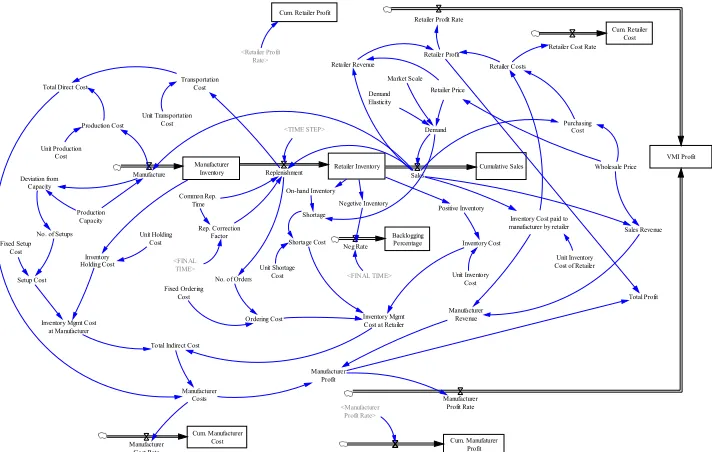
inventory costs paid by retailer. Similarly, inventory management cost at manufacturer’s side consists of inventory holding cost as well as setup costs once any setup cost is incurred. For more clarity, the setup cost will be considered merely if the retailer’s demand is less than the production capacity. In this case, manufacturer cannot produce the finished products continuously. Therefore, a production cost ( ) is being considered for each replenishment cycle. Beside the total indirect cost which is already discussed above, the manufacturer’s direct costs per unit time include transportation and production costs (See Figure 1 for more clarification). Likewise, the retailer’s profit can be simply obtained upon deduction of the retailer’s
costs from its revenues as it is shown in the SD model. Retailer’s revenue equals to the volume of products which are sold out to end customer on a retail price. On the other hand, retailer incurs purchasing cost on a wholesale price as well as the inventory cost that should be paid to manufacturer who is responsible for the overall inventory management of supply chain. Since in each time step of simulation model, we consider the total benefit of supply chain as the combined benefit of manufacturer and retailer, we preferably add two other state variables so as to be able to analyze the trend of cumulative benefit during a specific time horizon.
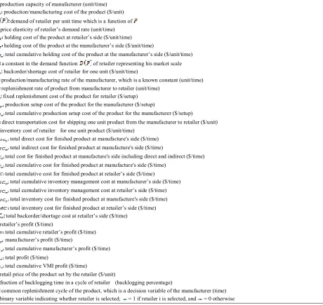
TABLE 1. Description of model variables and parameters
production capacity of manufacturer (unit/time) production/manufacturing cost of the product ($/unit)
demand of retailer per unit time which is a function of price elasticity of retailer’s demand rate (unit/time)
holding cost of the product at retailer’s side ($/unit/time) holding cost of the product at the manufacturer’s side ($/unit/time)
total cumulative holding cost of the product at the manufacturer’s side ($/unit/time) a constant in the demand function of retailer representing his market scale
backorder/shortage cost of retailer for one unit ($/unit/time)
production/manufacturing rate of the manufacturer, which is a known constant (unit/time) replenishment rate of product from manufacturer to retailer (unit/time)
fixed replenishment cost of the product for retailer ($/setup) production setup cost of the product for the manufacturer ($/setup)
total cumulative production setup cost of the product for the manufacturer ($/setup)
direct transportation cost for shipping one unit product from the manufacturer to retailer ($/unit) inventory cost of retailer for one unit product ($/unit/time)
total direct cost for finished product at manufacture's side ($/time) total indirect cost for finished product at manufacture's side ($/time)
total cost for finished product at manufacture's side including direct and indirect ($/time) total cumulative cost for finished product at manufacture's side ($/time)
total cumulative cost for finished product at retailer’s side ($/time)
total cumulative inventory management cost at manufacturer’s side ($/time) total cumulative inventory management cost at retailer’s side ($/time) total inventory cost for finished product at manufacture's side ($/time) total inventory cost for finished product at retailer’s side ($/time) total backorder/shortage cost at retailer’s side ($/time)
retailer’s profit ($/time)
total cumulative retailer’s profit ($/time) manufacturer’s profit ($/time)
total cumulative manufacturer’s profit ($/time) total profit ($/time)
total cumulative VMI profit ($/time)
retail price of the product set by the retailer ($/unit)
fraction of backlogging time in a cycle of retailer (backlogging percentage)
Demand Retailer Inventory Sales Manufacturer Inventory Manufacture Replenishment Market Scale Demand Elasticity Retailer Price Cumulative Sales Retailer Revenue Positive Inventory Common Rep. Time Transportation Cost Unit Transportation Cost Unit Production Cost Production Cost Fixed Setup Cost Unit Holding Cost Inventory Holding Cost Unit Inventory Cost Inventory Cost Unit Shortage Cost Shortage Cost Production Capacity Deviation from Capacity Total Direct Cost
Wholesale Price Purchasing
Cost
Unit Inventory Cost of Retailer Inventory Cost paid to manufacturer by retailer
No. of Orders
Retailer Profit
Inventory Mgmt Cost at Retailer Inventory Mgmt Cost
at Manufacturer
Total Indirect Cost
Manufacturer Revenue Manufacturer Profit Retailer Costs VMI Profit Retailer Profit Rate
Manufacturer Costs Ordering Cost Fixed Ordering Cost Rep. Correction Factor <FINAL TIME> Backlogging Percentage Neg Rate <FINAL TIME>
No. of Setups
Setup Cost <TIME STEP> Manufacturer Profit Rate Sales Revenue Cum. Manufaturer Profit <Manufacturer Profit Rate>
Cum. Retailer Profit
<Retailer Profit Rate> On-hand Inventory Shortage Negetive Inventory Total Profit Cum. Manufacturer Cost Manufacturer Cost Rate Cum. Retailer Cost Retailer Cost Rate
Figure 1. VMI basic SD model in VENSIM (Policy 1 or P1)
3. 3. Manufacturer Production Policies More commonly, manufacturers take the policy to produce the finished products with a fixed rate which is a function of end customer’s demand. Taking such policy into account, as far as the customer’s demand is bigger than manufacturer’s capacity, manufacturer is able to produce the finished products continuously with the same quantity of its capacity. Otherwise, due to the demand fluctuation, when the production capacity is redundant, he should adopt the required cost to setup the production line in a way to respond to market demand exactly with the same quantity requested. In contrast to this traditional policy (we call it P1) which is formerly addressed by Yu et al. [6], Almehdawe and Mantin [19], and Yu and Huang [20], we contribute to the current literature by the proposition of two other manufacturing policies hereinafter called P2 and P3. They are described as follows: Policy 2 (P2): Through this policy, we assume that the manufacturer can also contemplate the available inventory either in his storage or retailer’s stock to provide a better response to customer’s demand. In this case, manufacturer can use both capacities of production and on-hand inventories in stock to have a quick response for the market needs. In this policy, the effect of on-hand inventory either in manufacture's side or retailer’s side is reflected. In fact, we assume one additional variable called “available inventory” into the basic model of P1 as shown in Figure 2. As a result, the quantity of actual on-hand inventory also plays now a significant role in determination of manufacturing rate as well as the production capacity and market demand. In this case, manufacturing rate is being considered as a constant variable which should be determined as a function of
demand and inventory variables of both manufacturer and retailer.This policy and relevant mathematical “ IF-THEN” rules are already formulated for manufacturer. Establishment of such policy in a VMI partnership will decrease the replenishment of finished products to retailer while affecting the total profit of supply chain. Figure 2 illustrates the SD model of VMI supply chain for policy 2. To simplify the understanding of this figure, only the modified part of Figure 1 as the base model is presented (red color).
Figure 2. VMI SD model in VENSIM (Policy 2 or P2)
3. 4. Policy 3 (P3) Under this policy as shown in Figure 3, we have employed the advantages of learning theory using CKNN prediction algorithm. As earlier described, CKNN is one of the intuitive and practical algorithms being used for the classification and prediction in data mining and soft computing [44].
We assume these decision events and
corresponding manufacturing rates taken by manufacturer under the policies of P1 and P2 as the required synthetic dataset to execute policy P3. Therefore, using the CKNN and learning theory on the mentioned training dataset of past decisions, we can determine the optimum manufacturing rate in each time step from the nearest neighbor query results. As illustrated in Figure 3, the SD model for P3 has a minor change comparing with the basic one in a way that the manufacturing rate in this model is merely a function of a KNN variable i.e. none of the previous effective variables such as production capacity of manufacturer has no effect anymore. In this regard, we need to calculate the manufacturing rate in each time step of simulation by CKNN and reciprocally feed it as an input for SD model. Through CKNN, we firstly need to calculate the Euclidean distances for the dependent variables in each time step. This process will continue between CKNN and Vensim till simulation time finishes. Indeed, there should be a link or interface between CKNN module and Vensim. Therefore, we have developed a tool called OPTIMIZER by means of Delphi programming language and DLL functions of Vensim. The GUI of this application is illustrated in Appendix 1. Although we have faced with lots of programming constrains during the beginning of its development, it was followed by encouraging results at the end. It should be emphasized that in every run of SD model by Vensim to invoke a new manufacturing rate, the proposed CKNN algorithm should be reciprocally executed. This leads to find out the optimum manufacturing rate in each time step with the ultimate goal of increasing the total actual profit of supply chain. To find out the continuous k-nearest neighbors over the synthetic dataset of policies P1 and P2, we need to determine the CKNN variations. They include: (1) the number of neighbors to be revealed i.e. K or cardinality; (2) the similarity or distance metric to be used such as Euclidean, Manhattan, or Minkowski. In this paper, we use Euclidean which is the most common one in the literature. In this paper, the dependent variables to calculate the Euclidean distance include: "manufacturing rate", "manufacturer's inventory", and "retailer's inventory" which also play a significant role in determination of manufacturing rates in P2 ; (3) the combination strategy so as to determine the optimum manufacturing rate in each iteration. Herewith, we consider three types of combination functions including minimum distance, average, and weighted average.
TABLE 2. Primary values for the numerical example
adopted from Almehdawe and Odah [19].
Parameter Value
6
There are two other features that we have applied in our CKNN algorithm: 1. Normalization: to prevent the overwhelming of some variables that have large values in our calculations. Here, we use “min-max normalization”. The other available methods for normalization include z-score and decimal sampling; 2. Majority voting: in this regard, to find out the optimum manufacturing rate, we consider the most frequent classes among those of K nearby neighbors.
4. NUMERICAL EXAMPLE
For the numerical example, the primary input parameters are adopted from the optimal results of the work done by Almehdawe and Odah [19] as per listed in Table 2. The unit time is one month, the monetary unit is US dollar, and simulation time step in Vensim is 0.0625 of a month while the time horizon for simulation is 10 months.
4. 1. Performance and Sensitivity Analysis on
Execution of P1 and P2 According to the workflow mentioned in previous section, we initially execute the SD models of VMI with the policies of P1 and P2 by use of Vensim application. The results along with the sensitivity analysis for some selected parameters are presented in Table 3 (in two sections of 3-1 and 3-2 because of the limited space).
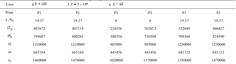
production in some cases i.e. a part of demand is compensated by the on-hand inventories available in both manufacturer and retailer stocks. Taking P2 into account, the related manufacturing costs are being decreased. The sensitivity analysis information shows by increasing the replenishment cycle from 3 months to 6 the total cumulative profit ( ) for both P1 and P2 decreases. Differently, the shipment of products in fewer cycles (from 3 to 1 month) increases the total cumulative profit. In addition, by limiting the production capacity ( ) of manufacturer from 200 to 100, the total cumulative profit for P1 is increased while we face no change for P2. With the decrease of market scale from to, the profit is decreased 24% and 20%, respectively for P1 and P2. This means changing the market scale needs to increase the production capacity as well. It is clear that less replenishment cycle in the VMI partnership in our case leads to have less shortage and backlogging.
4. 2. Execution of Policy P3 and Comparison
with P1 and P2 Now, we run P3 to evaluate and compare it with P1 and P2. Therefore, we start running of OPTIMIZER application to prepare the required synthetic dataset. As was discussed earlier, this necessitates execution of the first two policies. In this
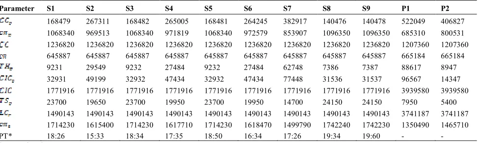
step, we build various scenarios on P3 so as to analyze the model from different perspectives. The scenarios are being built using multiple attributes including: the value of K as cardinality for nearest neighbors; the combination method (CM) which should be chosen from three available functions of minimum distance, average, and weighted average; and the option to include majority voting rule in relevant calculations or not. Therefore, we assume 9 different scenarios in our example which are described in Table 4.
The comparison results of S1 to S9 are summarized in Table 5. As the results show, the total VMI profit in P3 and its all 9 scenarios is much bigger than two previously discussed policies of P1 and P2. Among these 9 scenarios, S8 provides the biggest VMI profit. Our calculations show that the total profit increased about 29% and 19% respectively compared to P1 and P2. Although, total holding cost at manufacture's side ( ) of P3 in scenarios S1 to S7 are less than the same parameter of P1, but P2 provides better results in such cases. This parameter is optimized in S8 and S9 scenarios of P3 where we can see the lowest value of in S8 which is equal to 7386. The total backorder/shortage cost at retailer’s side ( ) in P3 has 60% decrease comparing with P1 and P2.
TABLE 3.1. Sensitivity analysis for the execution of P1 and P2 (Cases 1-3).
Case 1 Base 2 3
Prmt. P1 P2 P1 P2 P1 P2
19.37 19.37 56.25 56.25 0 0
522049 406827 1120000 1160000 296854 220338
685310 800531 84721.3 43384 910505 987020
1210000 1210000 1210000 1210000 1210000 1210000
665184 665184 665184 665184 665184 665184
1350000 1470000 750000 709000 1580000 1650000
TABLE 3.2. Sensitivity analysis for the execution of P1 and P2 (Cases 4-6).
Case 4 5 6
Prmt. P1 P2 P1 P2 P1 P2
19.37 19.37 0 0 19.37 19.37
407672 407118 224556 74307.5 522049 406827
799687 800241 580350 730598 709368 824590
1210000 1210000 805000 805000 1230000 1230000
665184 665184 443456 443456 641125 641125
1460000 1470000 1020000 1170000 1350000 1470000
TABLE 4. Specification of 9 different scenarios for P3.
Attribute Cardinality (K) Comb. method Majority voting
S1 3 Min. Dis. No
S2 3 Min. Dis. Yes
S3 3 Avg. No
S4 3 Avg. Yes
S5 3 W. Avg. No
S6 3 W. Avg. Yes
S7 6 Min. Dis. Yes
S8 10 Min. Dis. No
S9 10 W. Avg. No
TABLE 5. Results of different P3 scenarios besides the result of P1 and P2 policies.
Parameter S1 S2 S3 S4 S5 S6 S7 S8 S9 P1 P2
168479 267311 168482 265005 168481 264245 382917 140476 140478 522049 406827
1068340 969513 1068340 971819 1068340 972579 853907 1096350 1096350 685310 800531 1236820 1236820 1236820 1236820 1236820 1236820 1236820 1236820 1236820 1207360 1207360
645887 645887 645887 645887 645887 645887 645887 645887 645887 665184 665184
9231 29549 9232 27484 9232 27484 62748 7386 7387 88617 8947
32931 49199 32932 47434 32932 47434 77448 31536 31537 96567 14347
1771916 1771916 1771916 1771916 1771916 1771916 1771916 1771916 1771916 3939580 3939580
23700 19650 23700 19950 23700 19950 14700 24150 24150 7950 5400
1490143 1490143 1490143 1490143 1490143 1490143 1490143 1490143 1490143 3741187 3741187 1714230 1615400 1714230 1617710 1714230 1618470 1499790 1742240 1742230 1350490 1465710
PT* 18:26 15:33 18:34 17:35 18:50 16:34 17:26 19:34 19:60 - -
*Processing time
The comparison of S1 to S6 shows that with the same value for K=3 and without majority voting condition in S1, S3, and S5, there is no difference amongst the three combination methods since it is 1714230 for all of them. By the way, when the condition of majority voting is applied, the weighted average combination method provides bigger profit (1618470).
5. CONCLUSION, FUTURE WORKS AND
LIMITATIONS
In this paper, the dynamic behavior of a VMI supply chain and its key variables with three different manufacturing policies is studied. We developed a novel algorithm using simulation-based system dynamics and CKNN as a soft computing methodology. We used CKNN in our model so as to utilize the influence of learning and prediction in determination of manufacturing rate. A numerical study has been conducted to demonstrate how the proposed algorithms and policies are working. Besides, some sensitivity analysis are conducted. The proposed study can be extended in many directions: for example, the limiting assumptions of deterministic variables and parameters assumed in this paper could be generalized
to allow using of stochastic or fuzzy ones instead. Moreover, the number of retailers can be more i.e. the problem can be a single manufacturer multiple retailer or even more complex when we assume multiple manufacturer in place. Even, this limitation can be handled by means of subscript control function in Vensim DSS that allows modeling of multiple manufacturer and retailers distinctly. Other obvious extension to this work is to apply the other existing learning (and maybe forgetting) algorithms such as neural networks, regression, genetic algorithm, and etc. Consideration of a typical contract type such as consignment, buy-back, two-part tariff, or revenue sharing along with VMI can also be of additional line for future research.
6. REFERENCES
1. Rabelo, L., Helal, M. and Lertpattarapong, C., "Analysis of supply chains using system dynamics, neural nets, and eigenvalues", in Simulation Conference, Proceedings of the
2004 Winter, IEEE. Vol. 2, (2004), 1136-1144.
2. Al-Ameri, T.A., Shah, N. and Papageorgiou, L.G., "Optimization of vendor-managed inventory systems in a rolling horizon framework", Computers & Industrial
3. Disney, S.M. and Towill, D.R., "The effect of vendor managed inventory (vmi) dynamics on the bullwhip effect in supply chains", International Journal of Production Economics, Vol. 85, No. 2, (2003), 199-215.
4. Southard, P.B. and Swenseth, S.R., "Evaluating vendor-managed inventory (VMI) in non-traditional environments using simulation", International Journal of Production
Economics, Vol. 116, No. 2, (2008), 275-287.
5. Yao, Y., Evers, P.T. and Dresner, M.E., "Supply chain integration in vendor-managed inventory", Decision Support
Systems, Vol. 43, No. 2, (2007), 663-674.
6. Yu, Y., Chu, F. and Chen, H., "A stackelberg game and its improvement in a vmi system with a manufacturing vendor",
European Journal of Operational Research, Vol. 192, No. 3,
(2009), 929-948.
7. Zhao, Y., Wang, S., Cheng, T.E., Yang, X. and Huang, Z., "Coordination of supply chains by option contracts: A cooperative game theory approach", European Journal of
Operational Research, Vol. 207, No. 2, (2010), 668-675.
8. Cetinkaya, S. and Lee, C.-Y., "Stock replenishment and shipment scheduling for vendor-managed inventory systems",
Management Science, Vol. 46, No. 2, (2000), 217-232.
9. Darwish, M. and Odah, O., "Vendor managed inventory model for single-vendor multi-retailer supply chains", European
Journal of Operational Research, Vol. 204, No. 3, (2010),
473-484.
10. Wong, W.-K., Qi, J. and Leung, S., "Coordinating supply chains with sales rebate contracts and vendor-managed inventory", International Journal of Production Economics, Vol. 120, No. 1, (2009), 151-161.
11. Lertpattarapong, C., "Applying system dynamics approach to supply chain management problem", A Thesis Submitted to Massachusetts Institute of Technology, (2002).
12. Brown, G.G., Graves, G.W. and Ronen, D., "Scheduling ocean transportation of crude oil", Management Science, Vol. 33, No. 3, (1987), 335-346.
13. Disney, S.M., Potter, A.T. and Gardner, B.M., "The impact of vendor managed inventory on transport operations",
Transportation Research Part E: Logistics and
Transportation Review, Vol. 39, No. 5, (2003), 363-380.
14. Gurenius, P. and Wicander, J., "Vendor managed inventory (vmi): An analysis of how microsoft could implement vmi functionality in the erp system microsoft dynamics ax, Lund University, (2007).
15. Hennet, J.-C. and Arda, Y., "Supply chain coordination: A game-theory approach", Engineering Applications of Artificial
Intelligence, Vol. 21, No. 3, (2008), 399-405.
16. Holmstrom, J., "Business process innovation in the supply chain–a case study of implementing vendor managed inventory", European Journal of Purchasing & Supply
Management, Vol. 4, No. 2, (1998), 127-131.
17. Miller, D.M., "An interactive, computer-aided ship scheduling system", European Journal of Operational Research, Vol. 32, No. 3, (1987), 363-379.
18. Wang, W.-T., Wee, H.-M. and Tsao, H.-S.J., "Revisiting the note on supply chain integration in vendor-managed inventory", Decision Support Systems, Vol. 48, No. 2, (2010), 419-420.
19. Almehdawe, E. and Mantin, B., "Vendor managed inventory with a capacitated manufacturer and multiple retailers: Retailer versus manufacturer leadership", International Journal of
Production Economics, Vol. 128, No. 1, (2010), 292-302.
20. Yu, Y. and Huang, G.Q., "Nash game model for optimizing market strategies, configuration of platform products in a vendor managed inventory (vmi) supply chain for a product
family", European Journal of Operational Research, Vol. 206, No. 2, (2010), 361-373.
21. Achabal, D.D., McIntyre, S.H., Smith, S.A. and Kalyanam, K., "A decision support system for vendor managed inventory",
Journal of Retailing, Vol. 76, No. 4, (2000), 430-454.
22. Tyan, J. and Wee, H.-M., "Vendor managed inventory: A survey of the taiwanese grocery industry", Journal of
Purchasing and Supply Management, Vol. 9, No. 1, (2003),
11-18.
23. Kuk, G., "Effectiveness of vendor-managed inventory in the electronics industry: Determinants and outcomes", Information
& Management, Vol. 41, No. 5, (2004), 645-654.
24. Setak, M. and Daneshfar, L., "An inventory model for deteriorating items using vendor-managed inventory policy",
International Journal of Engineering-Transactions A:
Basics, Vol. 27, No. 7, (2014), 1081-1090.
25. Chen, J.-M., Lin, I. and Cheng, H.-L., "Channel coordination under consignment and vendor-managed inventory in a distribution system", Transportation Research Part E:
Logistics and Transportation Review, Vol. 46, No. 6, (2010),
831-843.
26. Ahmadvand, A., Asadi, H. and Jamshidi, R., "Impact of service on customers' demand and members' profit in supply chain",
International Journal of Engineering, Vol. 25, No. 3, (2012),
213-222.
27. Hafezalkotob, A. and Makui, A., "Modeling risk of losing a customer in a two-echelon supply chain facing an integrated competitor: A game theory approach", International Journal
of Engineering, Vol. 25, No. 1, (2012), 11-34.
28. Killingsworth, W.R., "Design, analysis and optimization of supply chains: A system dynamics approach, Business Expert Press, (2011).
29. Ashayeri, J. and Lemmes, L., "Economic value added of supply chain demand planning: A system dynamics simulation",
Robotics and Computer-Integrated Manufacturing, Vol. 22,
No. 5, (2006), 550-556.
30. Georgiadis, P., Vlachos, D. and Iakovou, E., "A system dynamics modeling framework for the strategic supply chain management of food chains", Journal of Food Engineering, Vol. 70, No. 3, (2005), 351-364.
31. Kamath, N.B. and Roy, R., "Capacity augmentation of a supply chain for a short lifecycle product: A system dynamics framework", European Journal of Operational Research, Vol. 179, No. 2, (2007), 334-351.
32. Rubiano Ovalle, O. and Crespo Marquez, A., "The effectiveness of using e-collaboration tools in the supply chain: An assessment study with system dynamics", Journal of
Purchasing and Supply Management, Vol. 9, No. 4, (2003),
151-163.
33. Ozbayrak, M., Papadopoulou, T.C. and Akgun, M., "Systems dynamics modelling of a manufacturing supply chain system",
Simulation Modelling Practice and Theory, Vol. 15, No. 10,
(2007), 1338-1355.
34. Georgiadis, P. and Besiou, M., "Sustainability in electrical and electronic equipment closed-loop supply chains: A system dynamics approach", Journal of Cleaner Production, Vol. 16, No. 15, (2008), 1665-1678.
35. Vlachos, D., Georgiadis, P. and Iakovou, E., "A system dynamics model for dynamic capacity planning of remanufacturing in closed-loop supply chains", Computers &
Operations Research, Vol. 34, No. 2, (2007), 367-394.
36. Minegishi, S. and Thiel, D., "System dynamics modeling and simulation of a particular food supply chain", Simulation
37. Kim, B. and Park, C., "Coordinating decisions by supply chain partners in a vendor-managed inventory relationship", Journal
of Manufacturing Systems, Vol. 29, No. 2, (2010), 71-80.
38. Lin, K.-P., Chang, P.-T., Hung, K.-C. and Pai, P.-F., "A simulation of vendor managed inventory dynamics using fuzzy arithmetic operations with genetic algorithms", Expert Systems
with Applications, Vol. 37, No. 3, (2010), 2571-2579.
39. Che, Z., "A particle swarm optimization algorithm for solving unbalanced supply chain planning problems", Applied Soft
Computing, Vol. 12, No. 4, (2012), 1279-1287.
40. Hajiaghaei-Keshteli, M., "The allocation of customers to potential distribution centers in supply chain networks: Ga and aia approaches", Applied Soft Computing, Vol. 11, No. 2, (2011), 2069-2078.
41. Ye, F. and Li, Y., "A stackelberg single-period supply chain inventory model with weighted possibilistic mean values under
fuzzy environment", Applied Soft Computing, Vol. 11, No. 8, (2011), 5519-5527.
42. Ko, M., Tiwari, A. and Mehnen, J., "A review of soft computing applications in supply chain management", Applied
Soft Computing, Vol. 10, No. 3, (2010), 661-674.
43. Han, J. and Kamber, M., Pei. Data mining concepts and techniques., The Morgan Kaufmann Series in Data Management Systems, Morgan Kaufmann Publishers., (2011). 44. Larose, D.T., "Discovering knowledge in data: An introduction
to data mining, John Wiley & Sons, (2014).
45. Zanoni, S., Jaber, M.Y. and Zavanella, L.E., "Vendor managed inventory (VMI) with consignment considering learning and forgetting effects", International Journal of Production
Economics, Vol. 140, No. 2, (2012), 721-730.
A Novel Continuous KNN Prediction Algorithm to Improve Manufacturing Policies
in a VMI Supply Chain
M. Akhbaria, Y. Zare Mehrjerdia, H. Khademi Zarea, A. Makuib
a Department of Industrial Engineering, Faculty of Engineering, Yazd University, Yazd, Iran b Department of Industrial Engineering, Iran University of Science and Technology, Tehran, Iran
P A P E R I N F O
Paper history:
Received 15 December 2013 Received in revised form 04 April 2014 Accepted 26 June 2014
Keywords:
Vendor Managed Inventory Continuous K-nearest Neighbor Learning, System Dynamics
هﺪﯿﮑﭼ
ﺖﮐاﺮﺷﮏﯾدﺮﮑﻠﻤﻋدﻮﺒﻬﺑﺖﻬﺟردﺪﻧاﻮﺗﯽﻣهﺪﻨﻨﮐﺪﯿﻟﻮﺗﮏﯾﻪﮐﺪﯿﻟﻮﺗﻒﻠﺘﺨﻣيﺎﻬﺘﺳﺎﯿﺳﻪﺴﯾﺎﻘﻣوﯽﺳرﺮﺑﻪﺑﻪﻟﺎﻘﻣﻦﯾا دزادﺮﭘﯽﻣﺪﻨﮐذﺎﺨﺗاهﺪﻨﺷوﺮﻓﻂﺳﻮﺗيدﻮﺟﻮﻣﺖﯾﺮﯾﺪﻣ .
ﺖﺳاﻦﯿﻣﺄﺗهﺮﯿﺠﻧزﯽﻌﻤﺠﺗوﯽﺒﯿﮐﺮﺗدﻮﺳندﻮﻤﻧ ﻢﻤﯾﺰﮐﺎﻣفﺪﻫ
ﯽﻌﺳﻪﮑﯿﻟﺎﺣرد دﻮﺷﻪﻨﯿﻤﮐﺰﯿﻧيدﻮﺟﻮﻣﺖﯾﺮﯾﺪﻣﻪﺑطﻮﺑﺮﻣيﺎﻫﻪﻨﯾﺰﻫدﻮﺷﯽﻣ
. ودهﺮﯿﺠﻧزﮏﯾﻪﻌﻟﺎﻄﻣدرﻮﻣﻦﯿﻣﺄﺗهﺮﯿﺤﻧز
يﺮﺳاﺮﺳﺖﯾﺮﯾﺪﻣﺖﯿﻟﻮﺌﺴﻣهﺪﻨﻨﮐ ﺪﯿﻟﻮﺗﻪﮑﯾرﻮﻄﺑ،ﺖﺳا ﺢﻄﺳﺮﻫردشوﺮﻓهدﺮﺧﮏﯾوهﺪﻨﻨﮐﺪﯿﻟﻮﺗﮏﯾﻞﻣﺎﺷﯽﺤﻄﺳ درادهﺪﻬﻋﺮﺑاريدﻮﺟﻮﻣ .
ﭘياﻪﯾﺎﭘويزﺎﺳﻪﯿﺒﺷلﺪﻣﮏﯾ،ﺖﺴﺨﻧﻪﻠﻫورد يﺎﯾﻮﭘتﻼﻣﺎﻌﺗﻒﯿﺻﻮﺗﺖﻬﺟردﻢﺘﺴﯿﺳﯽﯾﺎﯾﻮ
ﺖﺳاهﺪﺷﻪﺋاراهﺪﻨﺷوﺮﻓﻂﺳﻮﺗدﻮﺟﻮﻣﺖﯾﺮﯾﺪﻣيِﮋﺗاﺮﺘﺳاﺖﺤﺗشوﺮﻓهدﺮﺧوهﺪﻨﻨﮐﺪﯿﻟﻮﺗﻦﯿﺑيﺎﻫﺮﺘﻣارﺎﭘوﺎﻫﺮﯿﻐﺘﻣﻦﯿﺑ .
رﺎﺗﺪﻫدﯽﻣارهزﺎﺟاﻦﯾاﻪﮐهﺪﯾدﺮﮔدﺎﺠﯾاﺪﯿﻟﻮﺗهﺪﺷهرﺎﺷايﺎﻬﺘﺳﺎﯿﺳ،ﻢﺘﺴﯿﺳﯽﯾﺎﯾﻮﭘياﻪﯾﺎﭘلﺪﻣزاهدﺎﻔﺘﺳاﺎﺑﺲﭙﺳ يﺎﻫرﺎﺘﻓ
ﻢﯿﯾﺎﻤﻧﯽﺳرﺮﺑﺺﺨﺸﻣﯽﻧﺎﻣزهزﺎﺑﮏﯾﯽﻃارﺖﺳﺎﯿﺳﺮﻫﯽﻃهﺮﯿﺠﻧزيﺎﻀﻋاتوﺎﻔﺘﻣ .
ﻢﺘﯾرﻮﮕﻟازاهدﺎﻔﺘﺳاﺎﺑ،ﻪﻟﺎﻘﻣﻦﯾارد
k
ﻪﺘﺳﻮﯿﭘﯽﮕﯾﺎﺴﻤﻫﻦﯿﻣا )
CKNN ( يﺮﯿﮔدﺎﯾيﺎﻬﯾِژﻮﻟﺪﺘﻣزاﯽﮑﯾناﻮﻨﻌﺑ
-ﻢﯾزادﺮﭙﺑﺪﯿﻟﻮﺗخﺮﻧﻦﯾﺮﺘﻬﺑﯽﻨﯿﺑﺶﯿﭘﻪﺑرﻮﺤﻣ .
ﻦﯾا
ﺳﺮﮕﯾدﻪﺑﻪﺴﯾﺎﻘﻣردﻢﺘﯾرﻮﮕﻟا دﻮﺷﯽﻣهﺮﯿﺠﻧزدﻮﺳناﺰﯿﻣﺶﯾاﺰﻓاﻪﺑﺮﺠﻨﻣيﺮﺛﻮﻣزﺮﻄﺑﻪﻟﺎﻘﻣردهﺪﺷحﺮﻄﻣيﺎﻬﺘﺳﺎﯿ
. ﻦﯿﻤﻫرد
ﻢﯿﯾﺎﻤﻧﻪﺴﯾﺎﻘﻣارهﺪﺷﺮﮐذيﺎﻬﺘﺳﺎﯿﺳدﺮﮑﻠﻤﻋﺎﺗهﺪﯾدﺮﮔﻪﺋاراﺖﯿﺳﺎﺴﺣيﺎﻫﻞﯿﻠﺤﺗﺎﺑهاﺮﻤﻫيدﺪﻋلﺎﺜﻣﮏﯾ،ﺎﺘﺳار .
![TABLE 2. Primary values for the numerical example adopted from Almehdawe and Odah [19]](https://thumb-us.123doks.com/thumbv2/123dok_us/229859.2017561/6.595.309.529.121.342/table-primary-values-numerical-example-adopted-almehdawe-odah.webp)