IJE Transactions A: Basics Vol. 24, No. 1, January 2011 - 87
FREQUENCY ANALYSIS FOR A TIMOSHENKO BEAM
LOCATED ON AN ELASTIC FOUNDATION
M. Sadeghian
Department of Mechanical Engineering, Ferdowsi University of Mashhad Postal Code 9177948944-1111, Mashhad, Iran, [email protected]
H. Ekhteraei Toussi *
Department of Mechanical Engineering, Ferdowsi University of Mashhad Postal Code 9177948944-1111, Mashhad, Iran, [email protected]
*Corresponding Author
(Received: April 8, 2009 – Accepted in Revised Form: March 11, 2010)
Abstract It is quite usual to encounter a beam with different types of cross section or even structural discontinuities such as a crack along its length. Furthermore, in many occasions such a beam may happen to be exposed to the oscillatory fluctuations. Therefore, any information about its natural frequencies may be worthwhile. Amongst the problems of discontinues beam analysis, in this paper a special kind of frequency analysis for a cracked and stepped beam located on an elastic foundation is considered. Accordingly, following a look out at the definition of Timoshenko beams, a special modeling trend known as the wave method is introduced. Based on the d'Alembert’s approach for the solution of wave differential equations, the technique of wave method is mainly depended on the study of transmission and reflection of waves colliding to a barrier. The method results in a global frequency matrix, which its determinant gives out the natural frequencies. The wave method is employed for the frequency analysis in some kinds of cracked and stepped beams with different types of boundary conditions. In some typical cases, the results are compared to other similar works and confirmed to be convincing.
Key words Timoshenko beam, elastic foundation, Wave approach, Cracked stepped beam, Frequency analysis
ﻩﺪﻴﮑﭼ
ﺲﻧﺎـﮐﺮﻓﻪـﻌﻟﺎﻄﻣﺖـﻴﻤﻫﺍﻭﻮـﺴﮑﻳﺯﺍﺎـﻫﺮﻴﺗﻝﻮـﻃﺭﺩﺕﻭﺎﻔﺘﻣﯼﺭﺎﺘﺧﺎﺳﯼﺎﻫﯽﮕﺘﺳﻮﻴﭘﺎﻧﺩﻮﺟﻭﻞﻴﻟﺪﺑ
ﺮﮕﻳﺩﯼﻮﺳﺯﺍﺎﻫﺮﻴﺗﯽﻌﻴﺒﻃ ،
ﻊﻗﺍﻭﺭﺍﺪﮐﺮﺗﻭﻪﻠﭘﻮﮑﻨﺷﻮﻤﻴﺗﯼﺎﻫﺮﻴﺗﯽﻌﻴﺒﻃﺲﻧﺎﮐﺮﻓﺮﺑﺮﺛﻮﻣﻞﻣﺍﻮﻋﻪﻟﺎﻘﻣﻦﻳﺍﺭﺩ ﺮﺑ
ﺖﺳﺍﻩﺪﺷﯽﺳﺭﺮﺑﯽﻋﺎﺠﺗﺭﺍﺮﺘﺴﺑ
.
ﺎﺘﺳﺍﺭﻦﻳﺍﺭﺩ ﻦﻤﺿ
ﺢﻳﺮﺸﺗ ﻞﺣﻩﺍﺭ ﻮﺳﻮﻣ
ﺝﻮـﻣﺵﻭﺭﻪـﺑﻡ ،
ﻩﻮﻴـﺷ
ﺝﺍﺮﺨﺘـﺳﺍ
ﯼﺎﻫﺲﻧﺎﮐﺮﻓ ﯽﻌﻴﺒﻃ
ﻗﺍ ﺴ ﻪﺘﺳﻮﻴﭘﺎﻧﯼﺎﻫﺮﻴﺗﺯﺍﯽﻋﻮﻨﺘﻣﻡﺎ ﯽﻓﺮﻌﻣ
ﺖﺳﺍﻩﺪﺷ
.
ﺵﻭﺭﺭﺩ ﺝﻮﻣ
ﺵﻭﺭﻪـﺑﺎﮑﺗﺍﺎﺑ
ﻩﮋـﻳﻭ
ﻞﺣ ﺝﻮﻣﺕﻻﺩﺎﻌﻣ ﻪﺑﻡﻮﺳﻮﻣ
ﻞﺣ ﺮﺒﻣﻻﺍﺩ ،
ﯽـﺴﻳﺮﺗﺎﻣﻂـﺑﺍﻭﺭﻞﮑﺷﻪﺑﻊﻧﺍﻮﻣﺯﺍﺝﻮﻣﺱﺎﮑﻌﻧﺍﻭﺭﺬﮔﺎﺑﻂﺒﺗﺮﻣﺩﻮﻴﻗ
ﻢﻴﻈﻨﺗ ﻦﻳﺍﻪﻋﻮﻤﺠﻣﻕﺎﺤﻟﺍﺎﺑﻭﻩﺪﻳﺩﺮﮔ ﺩﻮﻴﻗ
، ﺪﻴﻟﻮﺗﯽﺴﻧﺎﮐﺮﻓﻞﻴﻠﺤﺗﯽﺳﺎﺳﺍﺲﻳﺮﺗﺎﻣ ﯽﻣ
ﺩﻮﺷ
.
ﻪﺸﻳﺭ
ﻥﺎـﻨﻴﻣﺮﺗﺩﯼﺎﻫ
ﯽﺳﺎﺳﺍﺲﻳﺮﺗﺎﻣ ،
ﺲﻧﺎﮐﺮﻓ ﺪﻨﺘﺴﻫﺮﻴﺗﯽﻌﻴﺒﻃﯼﺎﻫ
.
ﯼﺍﺮﺑﺝﻮﻣﻞﺣﺵﻭﺭﻪﻟﺎﻘﻣﻦﻳﺍﺭﺩ
ﻁﻮـﺑﺮﻣﯼﺎﻬﺴﻧﺎﮐﺮﻓﺝﺍﺮﺨﺘﺳﺍ
ﯽﻋﺎﺠﺗﺭﺍﺮﺘﺴﺑﺮﺑﻊﻗﺍﻭﯼﺎﻫﺮﻴﺗﻪﺑ ﺭﺍﺩﺮﻴﮔﺎﻳﯽﻠﺼﻔﻣ،ﺩﺍﺯﺁﻉﻮﻧﺯﺍﺕﻭﺎﻔﺘﻣﯽﻧﺍﺮﮐﻂﻳﺍﺮﺷﺎﺑ
ﻪﺋﺍﺭﺍ ﺖـﺳﺍﻩﺪﺷ
. ﺭﻮـﻄﺑ
ﻪﻧﻮﻤﻧ
ﺪـﻴﺋﺎﺗﺞﻳﺎـﺘﻧﺖﺤﺻﻭﻪﺴﻳﺎﻘﻣﺮﮕﻳﺩﯼﺎﻫﺵﻭﺭﺯﺍﻩﺪﻣﺁﺖﺳﺪﺑﯼﺎﻫﺦﺳﺎﭘﺎﺑﻞﺻﺎﺣﺞﻳﺎﺘﻧﺩﺭﺍﻮﻣﯽﺧﺮﺑﺭﺩ ﺖﺳﺍﻩﺪﺷ
.
1. INTRODUCTION
In the last decades due to the growing industrial need and in competition with experimental tests a tendency toward the analysis of vibration behavior of discontinues and cracked structures has been aroused. The presence of a crack in a structure
88 - Vol. 24, No. 1, January 2011 IJE Transactions A: Basics analyzed. The literature of vibration analysis is
filled with different analytical techniques for the analysis of free vibrations. Some types of these solution techniques include the using of the Finite Element Method [1-4], Galerkin and Ritz Method [5], approximate methods such as the one proposed in [6], transfer matrix method [7], dynamic stiffness matrix [8] and the methods given in [9] and [10] which are mainly based on the variational approaches in which one looks for a solution that optimizes a functional.
Using the d'Alembert's approach in the solution of differential equations of wave, the formulated technique of wave method is mainly based on the pursuit of the waves along the waveguides. In this method, one should follow the movements of waves, which transmit, reflect or propagate via the interior body barriers. The waves are divided to different types comprising of propagated, transmitted and reflected waves in waveguides [11-13]. Reflective and transitive features of waves are studied by different researchers [14-17]. The method of waves has recently used in an extensive level for the analysis of Timoshenko beam vibrations [18-21]. In line with this situation, in this paper different transmission and reflection matrices are derived for several types of discontinuities located in a Timoshenko beam placed on an elastic foundation. These discontinuities may include crack, change of cross section and even abrupt change of properties in the boundaries. By combining, these matrices a general method of solution for the analysis of free vibration of cracked Timoshenko beam located on elastic foundation can be obtained. To this ends, in the next section some minor wave matrices and the method of their synthesis are introduced. Natural frequencies of a structure are the roots of the determinant of its relevant synthesized wave matrix. In this paper, in order to find the roots of the frequency determinant a special algorithm of optimization is employed. The algorithm entitled as BFGS is named after its inventors Broyden, Fletcher, Goldfarb and Shanno [22] is briefly introduced in Section 4. So compared to the earlier works, the main advantages of this research are the inclusion of the foundation elasticity and another type of crack into the previous analyses, which in turn results in the wide range of revisions, and analyses for the determination of wave matrices.
Moreover, due to the complexity of the resulting wave equation, in the root finding stage a special solution technique is employed.
2. WAVE AND MOTION PROPAGATION
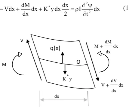
Subsequently the equations of motion of a beam on an elastic foundation considering the effects of shear deformation and rotary inertia are derived. The sum of the moments of all forces about the point O, in Figure 1 gives,
dx t I 2 dx dx y K dx dx dM
Vdx 2
2 *
(1)
The third term is negligible and can be ignored. So,
2 2
t I dx dM V
(2)
It is known that,
M(x, t) = EI ψ(x, t) x
(3)
and
x t) y(x, ) t , x ( GAk
) t , x ( V
(4)
Now, substituting Eqs. (3) and (4) in Eq.(2) gives,
V
M O
dx dx dM
M
dx dx dV V y
K*
dx
q(x)
IJE Transactions A: Basics Vol. 24, No. 1, January 2011 - 89 0 t t) (x, ρI t)] (x, xt) y(x, GAk[ x t) (x,
EI22 22
(5)
moreover, the balance of forces in the y direction
gives, 2 2 * t y ρAdx t)dx q(x, dx y K dx dx dV
. (6)
Similar formulas for the moment and force equilibrium but in the absence of foundation reaction can be found in [11].
Using Eq. (4) and Eq.(6) one obtains,
t) q(x, t t) y(x, ρA K ] x t) y(x, x t) (x, Ak[ G 2 2 * 2 2 y (7) Where x is the position along the beam axis, t is
the time, y(x,t) is the transverse deflection of the centre line of the beam, q(x,t) is the external force, E,G and are the Young’s modulus, shear modulus and mass density, K* is foundation flexibility, respectively. Moreover, I is the area moment of inertia of the cross section, A is the cross-sectional area, k is the shear coefficient of the beam, (x,t) is the slope due to bending,
x / t) y(x,
is the slope of the centerline of the beam and y(x,t)/x(x,t) is the shear angle. It can be seen that Eqs. (5) and (7) are coupled via
t)
ψ(x, and y(x,t) that are the slope and transverse deflection of the beam.
By using Eqs. (2) and (3) shear force V(x,t) at any section of the beam can be interrelated to the transverse deflection y(x,t) and slope ψ(x,t)as,
2 t t) (x, 2 ρI x t) ψ(x, EI t) V(x, 2 2
(8)
Some other requirements of this analysis are the three coefficients of Cb , Cs and Cr that will be used
in the next sections. The coefficients are proportional to the bending, shear and rotational stiffness respectively. They are,
ρA EI Cb ,
ρA GAk CS ,
ρA GJ
Cr (9)
The shear beam model, the Rayleigh beam model and the simple Euler–Bernoulli beam model can be obtained from the Timoshenko beam model by setting Cr equal to zero (that is, ignoring the
rotational effect), moving Cs to infinity (ignoring
the shear effect) and setting both Cr equal to zero
and Cs to infinity, respectively.
Assuming time harmonic motion and using separation of variables, the solutions to Eqs. (5) and (7) can be written as,
t iω
iKx
0
e
e
y
t)
y(x,
(10)and
t iω
iKx 0
e
e
t)
(x,
(11)where ω is the frequency and K is the wave number.
Substituting Eqs. (10) and (11) into Eqs. (5) and (7) gives,
0 0 0 ψ 0 y iKGAk KρAω
GAk K
ρIω
GAk EIK GAk iK * 2 2 2 2 (12) The determinant of matrix in Eq. (12) should
vanish. This gives a second-order polynomial in K2, which is,
0 ) EIGAk I K IA EI A K ( ) EI I GAk A K ( K K 2 * 4 2 2 * 2 2 * 2
4
(13) or simply, 0 c K b K
a0 4 0 2 0 (14)
Where
1
90 - Vol. 24, No. 1, January 2011 IJE Transactions A: Basics
GAk
K
K
K
b
* 2 2 b 2 1 b0
(14b)EIGAk
K
I
EI
K
K
K
c
* 2 * 2 2 b 2 1 b 0
(14c)Wherein
K
b1 andK
b2, i.e., the wave numbers ofthe tension free beam are,
4 2 2 b r 2 s 2 b 2 2 2 b r 2 s
b1 C) ω
C ( ) C 1 ( 4 1 C ω ω ) C C ( ) C 1 ( 2 1 K 4 2 2 b r 2 s 2 b 2 2 2 b r 2 s
b2 C ) ω
C ( ) C 1 ( 4 1 C ω ω ) C C ( ) C 1 ( 2 1 K
The solution to Eq. (12) gives a set of wave numbers which are functions of the frequency
(
)
as well as the properties of the structure, i.e.0 0 0 2 0 0 1 2a c 4a b b
K (14d)
0 0 0 2 0 0 2 2a c 4a b b
K (14e)
Here the () sign outside the brackets indicates that waves travel in both positive and negative directions along the beam.
The mode shape of the vibrating beam can now be derived by using of the K values in a linearly combination of the solution functions while at the same time the termeiω tshould be discarded. So the solution to Equations (5) and (7) can now be written as,
x K 2 x iK 1 x K 2 x iK 1 2 1 2
1 a e a e a e
e a
y(x)
(15a) x K 2 x iK 1 x K 2 x iK 1 2 1 2
1
a
e
a
e
a
e
e
a
(x)
(15b)
Clearly, the wave amplitudes (a) and ( a ) are related to each other. The relation can be found from Eq. (12) as,
KGAk K GAk K
ρAω
i y * 2 2 0
0
(16)
Thus, the relations between the coefficients of y(x) and ψ(x)are as follows:
N a a N, a a iP, a a iP, a a 2 2 2 2 1 1 1
1
(17)
In Eq. (17) P and N are,
GAk K K K 2 1 * 2 1 Aω 1
P (17a)
GAk K K Aω 1 K N 2 2 * 2 2 (17b)
Plus and minus signs show the right or left direction of the propagated wave, respectively.
3. PROPAGATION, REFLECTION, AND TRANSMISSION OF WAVES
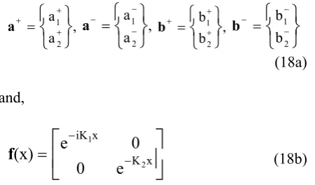
From the wave standpoint, any vibration propagating along a beam component will be reflected and transmitted upon discontinuities and boundaries. The propagation is governed by the so-called propagation matrix. Consider two points A and B on a vibrating uniform beam at distance x apart. Denoting the positive- and negative-going wave vectors at points A and B as a and
a
, and
b and b, respectively, they are related by
f b
a (x) ,
b
f
(x)
a
(18)IJE Transactions A: Basics Vol. 24, No. 1, January 2011 - 91
, a a 2 1 a
, a a 2 1 a
, b b 2 1 b
2 1 b b b (18a) and,
K xx iK 2 1
e
0
0
e
(x)
f
(18b)is known as the propagation matrix for a distance x.
The reflection and transmission characteristics of the waves are governed by the reflection and transmission matrices. A derivation of the reflection and transmission matrices at some discontinuities such as boundary barriers, cracks and cross-section changes are given in the following.
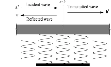
3.1. Reflections at the boundaries
A general boundary is shown in Figure 2. The incident wave
a
gives rise to the reflected wave
a . They are related by
r
a
a
(19)The reflection matrix
r
can be determined by considering the equilibrium at the boundary. That is ) t , x ( ψ K x t) ψ(x,EI R
(19a)
and the equilibrium of the forces results in,
) t , x ( y K ) t , x (
V T (19b)
Using (5) and (4) equation (19b) gives,
) t , x ( y K t) ψ(x,
ρIω
x t)
ψ(x,
EI 2 T
2 2
(20)
Where, K and T KRare the translational and
rotational stiffness of the support, respectively, and
x K 2 x iK 1 x K 2 x iK 1 2 1 2
1 a e a e a e
e a
y (21a)
x K 2 x iK 1 x K 2 x iK
1e 1 Na e 2 iPa e 1 Na e 2
iPa
.
(21b) If the boundary is at x = 0 , then the equilibrium
conditions become
0 a α a
α
12
11 (22)
Where T 2 2 2 T 2 2 1 R 2 R 1 11 K Iω Nρ NEIK K ω I ρ iP iPEIK NK EINK iPK EIPK α (22a) T 2 2 2 T 2 2 1 R 2 R 1
12 iPEIK iPρIω K NEIK NρIω K
NK EINK iPK EIPK α (22b) From Eqs. (19) and (22), it follows that
12 1 11 α α
r (23)
Three main boundary conditions are simply supported, clamped and free edge boundaries. Corresponding to these boundary conditions, K T and KR are either zero or infinite. The reflection matrices for simply supported, clamped and free
92 - Vol. 24, No. 1, January 2011 IJE Transactions A: Basics
1 0 0 1 s r iN P iN P iN P P 2 iN P iN 2 iN P iN P cr (24a)
22 f 21 f 12 f 11 ff
r
r
r
r
r
Where ) iK (K Iω ρ PN ) iK (K K EIPNK ) iK (K Iω ρ PN ) iK (K K EIPNK r r 2 1 2 1 2 2 1 2 1 2 1 2 2 1 f22 f11 ) iK (K Iω PNρ ) iK (K K EIPNK )ρINω
(EINK 2NK r 2 1 2 1 2 2 1 2 2 2 2 f12 ) iK (K Iω PNρ ) iK (K K EIPNK )
ρIPω
EIPK ( i2PK r 2 1 2 1 2 2 1 2 2 1 1 f21 (24b) 3.2. Crack
In this study, the local flexibility model is adopted from the Fracture Mechanics literature. In this approach the presence of crack is replaced by a local change in the beam flexibility [18]. In this work, the crack closure phenomenon, which encounters the crack edges tendency to remain closed despite the presence of an opening force, is neglected and the perpetually open crack model is assumed.
Considering an open single crack at x = 0 as shown in Figure 3 or similarly a double edge cracked beam as in Figure 4 a set of positive-going waves ais sent out towards the crack and gives rise to the transmitted and reflected waves
b and
a , which are related to the incident waves through the transmission and reflection matrices t
and r by
a t
b , a r a (25)
Denoting the transverse displacements and the slopes of the beam on the left- and right-hand sides
of the crack asy,y, ψandψrespectively, one has x K 2 x iK 1 x K 2 x iK
1e 1 a e 2 a e 1 a e 2
a
y (26a)
x K 2 x iK 1 2 1 b e
e b
y (26b)
x K 2 x iK 1 x K 2 x iK 1 2 1 2
1 Na e iPa e Nae
e iPa
ψ (27a)
x K 2 x iK 1 2 1 Nb e e
iPb
ψ (27b)
Since the beam is continuous, one has
y
y ,ψ ψCEI(ψ/x) (28) Figure 3. Single edge cracked beam.
IJE Transactions A: Basics Vol. 24, No. 1, January 2011 - 93
where the term CEI(ψ/x)represents a jump in the bending slope caused by the local flexibility change at the crack and C is the so-called flexibility coefficient. As in [19] C is related to the crack size (μ), which is the ratio between the depth of the crack and the thickness of the beam, i.e. ) μ f( EI )h ν (1 6Π C 2
(29)
Based on [19] f(μ)in Eq. (29) for the single edge crack
00.6
can be given by,10 9 8 7 6 5 4 3 2 μ 19.6 μ 40.7556 μ 47.1063 μ 33.0351 μ 20.2948 μ 9.973 μ 4.5948 μ 1.0533 μ 0.6272 ) μ f( (29a) and similarly for the double edge cracked beam
where
00.3
it can be given by,16 12 11 10 9 8 7 6 5 4 3 2 μ 42308 . 5 μ 93036 . 6 μ 7367 . 9 μ 55976 . 2 μ 3391 . 2 μ 49091 . 2 μ 33244 . 7 μ 55301 . 7 μ 17738 . 5 μ 72015 . 3 μ 03508 . 1 μ 63845 . 0 ) μ f( (29b)
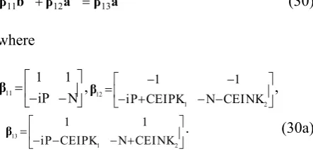
Using the continuity conditions in matrix form, one obtains,
β a β a
b
β11 12 13 (30)
where N iP 1 1 11
β ,
2 1
12 iP CEIPK N CEINK 1 1 β , 2 1 13 K N I E C N K P I E C P i 1 1
β . (30a)
Furthermore, by considering the equilibrium of the support,
V
V , M M (31)
One has a β a β b
β21 22 23 (32)
where N) K GAk( iP) iK GAk( EINK EIPK 2 1 2 1 21 β , N) K GAk( iP) iK GAk( EINK EIPK 2 1 2 1 22 β , N) K GAk( iP) iK GAk( EINK EIPK 2 1 2 1 23
β . (32a)
Eqs. (25), (30) and (32) can be solved to obtain the reflection and transmission matrices at the crack discontinuity as
13
1 12 22 23 11 1 12 22 21 1 t ,
22 21 111 12
23 21 111 13
1 β β β β β β β β
r . (33)
3.3. Change in section
As shown in Figure 5 let two beams of different properties be joined at x = 0 . Due to the mismatch of impedances, the incident waves from one side, give rise to the reflected and transmitted waves at the junction.
However, the displacement, slope, bending moment and shear force are all continuous at the
94 - Vol. 24, No. 1, January 2011 IJE Transactions A: Basics junction. The reflection and transmission matrices
can then be obtained from the continuity and equilibrium conditions.
Denoting the parameters related to the incident and transmitted sides of the junction with the subscripts L and R, respectively, choosing the origin at the point where the section changes, at
x = 0 , one has
R
L y
y ,ψL ψR,VL VR,ML MR (34) Using Eqs. (25), Eqs. (34) can be put into a matrix form in terms of the reflection and the transmission matrices rLL andtLR:
13 LR 12 LL
11r γ t γ
γ (35a)
23 LR 22 LL
21r γ t γ
γ (35b)
where
, N iPL L
1 1
11 γ
, N iP
1 1
R R 12
γ
, N iP
1 1
L L 13
γ
L L L1 L L L2
2 2 2 2
21
L L L1 L L L L2 L
(EI) P K -(EI) N K
γ = ,
i(EI) P K - iρIω P -(EI) N K -ρ Iω N
R R R1 R R R2
2 2 2 2
22
R R R1 R R R R2 R
-(EI) P K (EI) N K
γ = ,
i(EI) P K - iρ Iω P -(EI) N K -ρIω N
L L L1 L L L2
2 2 2 2
23
L L L1 L L L L2 L
-(EI) P K (EI) N K
γ = .
i(EI) P K - iρ Iω P -(EI) N K -ρIω N
(35c) The equations can be solved for the reflection and
transmission matrices rLL andtLR, which provides,
23
1 22 13 1 12 21 1 22 11 1 12 LL
1
γ γ γ γ γ γ γ γ
r ,
23
1 21 13 1 11 1 22 1 21 12 1 11
LR γ γ γ γ γ γ γ γ
t (36)
4. BFGS OPTIMIZATION ALGORITHM
An important stage of this work was the solution of the frequency equation. Due to the complexity of the frequency equation, its solution demanded special root finding techniques. Consequently, based on some examinations an optimization technique was selected for the root finding stage. The selected method entitled as BFGS (named after its inventors Broyden-Fletcher-Goldfarb-Shanno [21]) is the technique, which rapidly converges to the solution. The method is an enhanced version of the Newton optimization technique.
In an optimization problem, a multivariable objective function such as F(X) should be minimized. Here the main ambition is to find a proper optimal vector X such that the n variable objective function F becomes minimized. To introduce the method, let us primarily reconsider the structure of Newton's method. In Newton Method, a truncated approximation of the Taylor series around the point Xk is used. It results in,
T k 1
k k
1
k
X
[
H
(
X
)]
F
(
X
)
X
(37)
Where H(Xk)is the Hessian matrix, i.e. the second derivative or
2F
(X
k)
of a function F in a pointXk. However, in BFGS, in each step the Hessian matrix is approximated by a formula as,
k k BFGS
1
k
H
N
H
(38)IJE Transactions A: Basics Vol. 24, No. 1, January 2011 - 95
ω ) Im( EI) ω ( Re ER
A A
(39)
Assuming a new variable TE as, TEER2EI2 to
find the roots of the A() one may try to find the extremum value of TE, which at the same time is the root of the wave matrix.
5. VIBRATION ANALYSIS USING WAVE METHOD
The reflection and transmission matrices for the waves passing a discontinuity located along a beam are obtained in the preceding sections. To prepare the global wave matrix of a problem this matrices must be combined. To find the natural frequencies of the beam the determinant of this matrix should be vanished. In this paper in order to assess the method this procedure of finding natural frequencies will be verified on the beams having single or double edge cracks and the beams with stepped change in their cross sections. Now some typical applications of the systematic solution method for the analysis of free vibration of simply supported and cracked beams are given. The physical parameters of the beam are shown in Table (1)
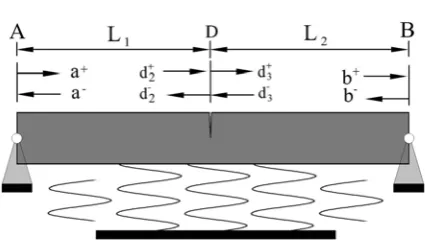
Figure 6 depicts a cracked beam assumed to have uniform cross section and its deformation pattern obeys the model of Timoshenko beam. A geometrical discontinuity is located at D. The
incident and reflected waves across the A and B support a and on both sides of the D crack are shown as
a
,b
,d
2 ,
3
d
.The connection between the incident and reflected waves in the boundaries are described by the following equations:
a
r
a
a (40a)
r
b
b
b (40b)In the geometrical discontinuity located in D the incident and reflected waves are related as,
2 3
3 rd td
d (41a)
2 3
2 rd td
d (41b)
In which the reflection and transmission matrices are given in section 3 and Propagation relationships are:
b f
d3 (L2) (41c)
3 2)
(L d f
b (41d)
2 1)
(L d f
a (41e)
Figure 6. Cracked simply supported beam
Table 1. The parameters of the sample cracked beam
Elastic const: E(GPa)
Shear factor: k
Poisson’s
ratio:
b(m) Width: 72 5.6 0.35 0.006 Thickness:h(m)
Length: L(m)
Density:
96 - Vol. 24, No. 1, January 2011 IJE Transactions A: Basics
a f
d2 (L1) (41f)
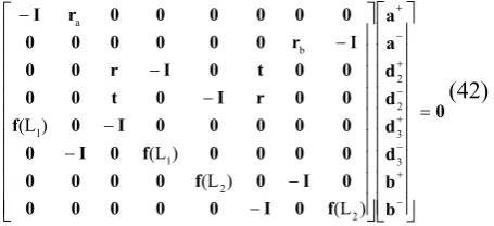
In which f(L1) and f(L2) are the propagation matrices between AD and DB. In matrix form the equations can be reshaped as,
0
b b d d d d a a
f 0 I 0 0 0 0 0
0 I 0 f 0 0 0 0
0 0 0 0 f 0 I 0
0 0 0 0 0 I 0 f
0 0 r I 0 t 0 0
0 0 t 0 I r 0 0
I r 0 0 0 0 0 0
0 0 0 0 0 0 r I
3 3 2 2
2 2
1 1
b a
) (L )
(L ) (L )
(L
(42)
To find a nontrivial solution for the variable
as the natural frequency of cracked Timoshenko beam the determinant of A matrix should vanish. The natural frequencies of the respected beam with and without a crack are studied in the following section.Case 1. Single edge cracked beam
Assuming different stiffness factor for the foundation and different crack length i.e.
00.6
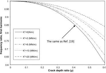
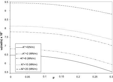
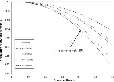
a variety of calculations have been done to show the variation of natural frequency of the defined beam in different instances.As can be seen in Figure 7 the more is the stiffness of the foundation the more will be the natural frequency of the whole beam while as usual the deeper crack results in a lower beam frequency. Figure 8 is the normalized type of Figure 7. A similar graph to Figure 8 can be found in [19], which shows a close agreement to this work.
In Figure 9 the Influence of foundation flexibility upon the natural frequency of the cracked beam is represented. Based on the results given [20] it is expected that the change in foundation flexibility have mostly effective on the lower frequencies. Figure 9 backs up this anticipation.
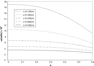
Now the effect of beam length on the natural
frequency of the beam is studied.
Figure 10 reveals that the more is the length of the beam the less will be its natural frequency. The Figure also shows that the effect of crack length in short beams is more severe than in long beams.
In this part, the effect of crack position (L1) upon the natural frequencies is studied. In order to do this, different cracks are placed in different locations on the beam and the first natural frequency of the cracked beam is calculated.
Based on Figure 11 when crack is near the beam support, the natural frequency of the beam is less than a middle length cracked beam.
Case 2. Double edge cracked beam
Assuming different stiffness factor for the foundation and different crack length i.e.
00.3
a variety of calculations have been done to show the variation of natural frequency of the beam in different instances.As it can be seen in Figure 12 the more is the stiffness of the foundation the more is the natural frequency of the whole beam while as usual the deeper crack results in the lower beam frequencies. Fig. 13 is the normalized type of Figure 12.
A similar graph to Figure 13 can be found in [19], which show a close agreement.
Now the effect of the beam length on the natural frequencies is studied.
Figure 14 reveals that the more is the length of the beam the less will be its natural frequency. The Figure also shows that the effect of crack length in short beams is more severe than in long beams.
Once again, in this part the effect of crack position (L1) on the natural frequencies is studied. In order to do this, crack is assumed to be placed in different locations on the beam and the first natural frequencies of the cracked beam are calculated.
Based on Figure 15 when crack is close to the beam support the natural frequency of the beam is less than a mid-length cracked beam.
IJE Transactions A: Basics Vol. 24, No. 1, January 2011 - 97 3.8
4.8 5.8 6.8 7.8 8.8
0 0.1 0.2 0.3 0.4 0.5 0.6
μ
ω
(r
ad/s) X
10
3
3 K*=0(N/m)
K*=2 (MN/m)
K*=8 (MN/m)
K*=10 (MN/m)
K*=20 (MN/m)
Figure 7. First natural frequency of the single edge cracked simply supported beam versus the crack depth ratio for different foundation flexibilities.
0.6 0.65 0.7 0.75
0.8 0.85
0.9 0.95
1
0 0.1 0.2 0.3 0.4 0.5 0.6
Crack depth ratio (µ)
fr
eque
nc
y r
a
ti
o
, f
ir
s
t
ha
rm
o
n
ic
K*=0(N/m)
K*=2 (MN/m)
K*=8 (MN/m)
K*=10 (MN/m)
K*=20 (MN/m)
The same as Ref. [19]
98 - Vol. 24, No. 1, January 2011 IJE Transactions A: Basics
0 10 20 30 40 50 60
0 2 4 6 8 10 12 14 16 18 20
ω1(rad/s)
ω2(rad/s)
ω3(rad/s)
ω
(rad/s)
x 1
0
3
K*(MN/m)
Figure 9. The first three natural frequencies of the single edge cracked simply supported beam versus the foundation flexibility.
0 2 4 6 8 10
12 14 16
18
20
0 0.1 0.2 0.3 0.4 0.5 0.6
µ
ω
(r
a
d
/s) x 1
0
3
L=0.135(m) L=0.185(m) L=0.235(m) L=0.285(m) L=0.335(m)
IJE Transactions A: Basics Vol. 24, No. 1, January 2011 - 99
3.75 4.25 4.75 5.25 5.75 6.25 6.75
0 0.1 0.2 0.3 0.4 0.5
µ
ω
(r
a
d
/s) x 1
0
3
L1=(L/2)
L1=(L/3)
L1=(L/4)
L1=(L/5)
L1=(L/6)
0.6
Figure 11. First natural frequency of the single edge cracked simply supported beam versus the crack depth ratio for different relative crack position.
5.5 6 6.5 7 7.5 8 8.5 9 9.5
0.05 0.1 μ 0.15 0.2 0.25 0.3
ω
(ra
d
/s
) x
1
0
3
K*=0(N/m)
K*=2 (MN/m)
K*=8 (MN/m)
K*=10 (MN/m)
K*=20 (MN/m)
0
100 - Vol. 24, No. 1, January 2011 IJE Transactions A: Basics Now the effect of crack position for two
different types of cracked beams is studied. In one case, the beam is a single edge cracked beam while in the other case a beam with similar shape, material and boundary condition except for the shape of the crack is considered. For the former one the beam is taken to be a double edge cracked beam such that both cracks are equal in length, total length of the cracks is equal to the crack length of a single edge cracked beam, and that cracks are located in a line perpendicular to the beam axis. The graph shows that in this case a double edge beam has greater natural frequency.
In this stage the natural frequency of the beams with length L (for the single edge cracked beam) and L' (for the double edge cracked beam) are compared.
Figure 17 shows that in single edge cracked beam the length effect on the natural frequency is more severe than in a similar double edge cracked beam.
Now the effect of foundation flexibility, K*, is studied. In the graphs, the sign K' designates a data
point for the natural frequency of a double edge cracked beam while the simple K sign introduces a single edge cracked beam natural frequency.
Here also it can be seen that in similar conditions the natural frequency of a single edge cracked beam is lower than a double edge cracked one.
Based on the results given in Figures, It can be seen that the presence of a crack on a beam can reduce natural frequency of the beam. Thus the crack presence works as like as the increase of structural flexibility or compliance. The increase of the crack and beam lengths can increase the flexibility of the beam. While increasing the proportion of crack position symmetry relative to the beam axis as well as the foundation flexibility decreases the flexural stiffness.
Notice that in this manner a single edge cracked beam is assumed less symmetric than a double edge cracked beam. All the natural frequencies obtained by this method for the beams without any crack are similar to the results given in reference [23]. Note that in Figure (7) the
0.84 0.86 0.88 0.9 0.92
0.94 0.96
0.98 1
0 0.1 0.2 0.3 0.4 0.5 0.6
Fr
eque
nc
y r
a
ti
o,
f
ir
s
t h
a
rm
o
n
ic
K*=0(N/m)
K*=2 (MN/m)
K*=8 (MN/m)
K*=10 (MN/m)
K*=20(MN/m)
Crack depth ratio The same as Ref. [19]
IJE Transactions A: Basics Vol. 24, No. 1, January 2011 - 101
0 2 4 6 8 10 12 14 16 18 20
0 0.05 0.1 0.15 0.2 0.25 0.3
μ
ω
(r
a
d
/s
) x
10
3
L=0.135(m)
L=0.185(m)
L=0.235(m)
L=0.285(m)
L=0.335(m)
Figure 14. First natural frequency of the double edge cracked simply supported beam versus crack depth ratio for different beam lengths.
5.5 5.7 5.9 6.1 6.3 6.5
0 0.05 0.1 0.15 0.2 0.25 0.3
μ
ω
(r
ad/s) x
1
0
3
L1=(L/2)
L1=(L/3)
L1=(L/4)
L1=(L/5)
L1=(L/6)
102 - Vol. 24, No. 1, January 2011 IJE Transactions A: Basics
3.75
4.25
4.75
5.25
5.75
6.25
6.75
0 0.1 0.2 0.3 0.4 0.5 0.6
ω
(rad/
s) x
1
0
3
L1’=(L/2)
L1=(L/2)
L1’=(L/3)
L1=(L/3)
L1’=(L/4)
L1=(L/4)
L1’=(L/5)
L1=(L/5)
L1’=(L/6)
L1=(L/6)
μ
Figure 16. A comparison between the natural frequencies of the single and double edge cracked simply supported beam versus the crack depth ratio for different relative crack positions.
2 4 6 8 10 12 14 16 18 20
0 0.1 0.2 0.3 0.4 0.5 0.6
µ
ω
(ra
d
/s) x
1
0
3
L'=0.135(m) L=0.135(m) L'=0.185(m) L=0.185(m) L'=0.235(m) L=0.235(m) L'=0.285(m) L=0.285(m) L'=0.335(m) L=0.335(m)
IJE Transactions A: Basics Vol. 24, No. 1, January 2011 - 103
intersections between the curves and the ordinate pinpoint the natural frequencies of a crack-free beam, which can similarly be obtained by the formulas derived in the foresaid Ref. [23].
Example 2. A stepped beam with a crack
Figure 19 shows a cracked stepped Timoshenko beam. The stepwise discontinuity is located at point E. The analysis follows the same procedures described above, except that there is additional wave reflection and transmission at the step change. Waves on both sides of the step discontinuity are related as the following:
4 RL 3 LL
3 r e t e
e ,e4 rRRe4 tLRe3 (43) The subscripts of r and t identify the incident and transmitted sides of the junction. The propagation relations are redefined as
f a
d2 (L1) ,a f(L1)d2,
3 2 3 f(L )d
e ,
3 2 3 f(L )e
d ,b f(L3)e4,e4 f(L3)b (44)
Where f(L1), f(L2)and f(L3)are the propagation matrices between AD, DE and EB, respectively. Writing Eqs. (37), (43) and (44) in matrix form results in Eq. (45).
Eq. (46) gives the characteristic equation from which the natural frequencies of cracked and stepped Timoshenko beams can be found. Using Eq. (46) the algorithm of the computer code is
Figure 19. A cracked stepped simply supported beam.
3.5 4.5 5.5 6.5 7.5 8.5 9.5
0 0.1 0.2 0.3 0.4 0.5
µ
ω
(rad
/s) x
1
0
3
K*'=0(N/m) K*=0(N/m)
K*'=2(MN/m)
K*=2 (MN/m) K*'=8 (MN/m) K*=8 (MN/m) K*'=10 (MN/m) K*=10 (MN/m) K*'=20(MN/m)
K*=20(MN/m)
0.6
104 - Vol. 24, No. 1, January 2011 IJE Transactions A: Basics a b LL RL LR RR 1 1 2 2 3 3
-I r 0 0 0 0 0 0 0 0 0 0
0 0 0 0 0 0 0 0 0 0 r -I
0 0 r -I 0 t 0 0 0 0 0 0
0 0 t 0 -I r 0 0 0 0 0 0
0 0 0 0 0 0 r -I 0 t 0 0
0 0 0 0 0 0 t 0 -I r 0 0
f(L ) 0 -I 0 0 0 0 0 0 0 0 0
0 -I 0 f(L ) 0 0 0 0 0 0 0 0
0 0 0 0 f(L ) 0 -I 0 0 0 0 0
0 0 0 0 0 -I 0 f(L ) 0 0 0 0
0 0 0 0 0 0 0 0 f(L ) 0 -I 0
0 0 0 0 0 0 0 0 0 -I 0 f(L )
+ -+ 2 -2 + 3 -3 + 3 -3 + 4 -4 + -a 0 a 0 d 0 d 0 d 0 d 0 = 0 e 0 e 0 e 0 e 0 b 0 b (45) 0 3 3 2 2 1 1 ) (L ) (L ) (L ) (L ) (L ) (L RR LR RL LL b a f 0 I 0 0 0 0 0 0 0 0 0 0 I 0 f 0 0 0 0 0 0 0 0 0 0 0 0 f 0 I 0 0 0 0 0 0 0 0 0 0 I 0 f 0 0 0 0 0 0 0 0 0 0 0 0 f 0 I 0 0 0 0 0 0 0 0 0 0 I 0 f 0 0 r I 0 t 0 0 0 0 0 0 0 0 t 0 I r 0 0 0 0 0 0 0 0 0 0 0 0 r I 0 t 0 0 0 0 0 0 0 0 t 0 I r 0 0 I r 0 0 0 0 0 0 0 0 0 0 0 0 0 0 0 0 0 0 0 0 r I (46)
revised, the values of natural frequencies of a double edge cracked, and stepped beam are calculated. In this case, the crack is still assumed to be at 0.5L and the step change occurs at 0.75L. Using a step size or a degree of precision of
0.001 rad/sec for the root finding of the characteristic equation given in (46) the values of natural frequencies are calculated and its results for sample values of foundation flexibility and crack length are displayed in Figure 20. The figure shows that decreasing the cross section results in the decrement of the natural frequency.
6. Conclusion
In this paper, the wave method approach is used for the free vibration analysis of a Timoshenko beam located on an elastic foundation with structural discontinuities in the shape of stepwise cross section change or an open edge crack. In order to perform this analysis different matrices of reflection, transmission and propagation are obtained and used to construct a global frequency matrix. To find the roots of the frequency matrix determinant a computer code has been devised which is based on the optimization technique of BFGS.
The implicated code is verified by the solution of a few benchmarking problems. Different examples are picked out and solved to show the effect of the factors such as the crack type or position, change of cross section and foundation flexibility. For example, the results reveal that a crack in the middle of a beam is more influential than a crack near by a beam support and the reduction of cross section results in the decrease of the beam natural frequency and that the stiff foundation gives up high natural frequencies.
7. Nomenclature:
A beam cross-sectional area (m2)
B width (m)
C local crack flexibility (1/Nm) Cr rotational stiffness coefficient
Cs shear stiffness coefficient
Cb bending stiffness coefficient
E Young modulus (N/m2)
G shear modulus (N/m2)
H depth of beam(m)
I area moment of inertia (N/m2)
IJE Transactions A: Basics Vol. 24, No. 1, January 2011 - 105
k shear coefficient KT translational stiffness (N/m)
KR rotational stiffness (N/m)
K* foundation flexibility L length of beam (m) M bending moment (Nm) T time (sec)
V shear force (N)
y(x,t) lateral displacement function
t) (x,
lateral slop function
natural frequencies of beam(Hz)
Poisson's ratio µ crack ratio material density(kg/m3)
8. REFERENCES
1. Dimarogonas, A.D., " Vibration of cracked structures: a state of the art review", Engineering Fracture Mechanics vol. 5, (1996), 831–857.Remley, T. J.,
Abdel-Khalik, S. I., Jeter, S. M., Ghiaasiaan, S. M. and Dowling, M. F., “Effect of Non-Uniform Heat Flux on Wall Friction and Convection Heat Transfer Coefficient in a Trapezoidal Channel”, International Journal of Heat and Mass Transfer, Vol. 44, (2001), 2453-2459.
2. Cawley, P. and Adams, R.D. "Structures from measurements of natural frequencies", Journal of Strain Analysis vol. 14, (1979), 49–57.
3. Krawczuk, M. and Ostachowicz, W.M., "Modeling and vibration analysis of a cantilever composite beam with a transverse open crack", Journal of Sound and Vibration vol. 183, (1995), 69–89.
4. Nandwana, B.P. and Maiti, S.K., "Detection of the location and size of a crack in stepped cantilever beams based on measurements of natural frequencies", Journal of Sound and Vibration vol. 203, (1997), 435–446.
5. Shen, M.H.H. and Pierre, C., "Free vibration of beams with a single-edge crack", Journal of Sound and Vibrationvol. 170, (1994), 237–259.
6. Narkis, Y., " Identification of crack location in vibrating simply supported beams", Journal of Sound and Vibration vol. 172, (1994), 549–558.
7. Tsai, T.C. and Wang, Y.Z., "Vibration analysis and diagnosis of a cracked shaft", Journal of Sound and Vibration vol. 192, (1996), 607–620.
8. Khiem, N.T. and Lien, T.V., "The dynamic stiffness
matrix method in forced vibration analysis of multiple-cracked beam", Journal of Sound and Vibration vol.
254, (2002), 541–555.
9. Behzad M., Meghdari A., Ebrahimi A., "A new approach for vibration analysis of a cracked beam", International Journal of Engineering vol. 18, No. 4 (2005) 319-330.
10. Ranjbaran A., Hashemi S. and Ghaffarian A. R., "A new approach for buckling and vibration analysis of a cracked beam", International Journal of Engineering vol. 21,
No. 3 (2008) 225-230.
11. Graff, K.F., "Wave Motion in Elastic Solids", Ohio State University Press, Ohio, 1975.
12. Cremer, L. and Heckel, M. and Ungar, E.E., "Structure-Borne Sound", Springer, Berlin, 1987
13. Doyle, J.F., "Wave Propagation in Structures", Springer,
New York, 1989.
14. Mace, B.R., "Wave reflection and transmission in beams", Journal of Sound and Vibration vol. 97,
(1984), 237–246.
15. Tan, C.A., and Kang, B., "Wave reflection and transmission in an axially strained, rotating Timoshenko shaft", Journal of Sound and Vibration vol. 213,
(1998), 483–510.
16. Harland, N.R. and Mace, B.R. and Jones, R.W., "Wave propagation, reflection and transmission in tunable fluid-filled beams", Journal of Sound and Vibration vol. 241,
(2001), 735–754.
17. Mei, C. and Mace, B.R., "Wave reflection and transmission in Timoshenko beams and wave analysis of Timoshenko beam structures", ASME Journal of Vibration and Acoustics vol. 127, (2005), 382–394.
18. Chondros, T.G., "The continuous crack flexibility model for crack identification", Fatigue and Fracture of Engineering Materials and Structures vol. 24, (2001),
643–650.
19. Chondros, T.G. and Dimarogonas, A.D. and Yao, J., "A continuous cracked beam vibration theory", Journal of Sound and Vibration vol. 215, (1998), 17–34.
20. Ming-Hung, Hsu., "Vibration Characteristics of Rectangular Plates Resting on Elastic Foundations and Carrying any Number of Sprung Masses" , International Journal of Applied Science and Engineering vol. 4,
(2006) 83-89.
21. Mei, C. and Karpenko, Y. and Moody, S. and Allen, D., "Analytical approach to free and forced vibrations of axially loaded cracked Timoshenko beams", Journal of Sound and Vibration vol. 291, (2006), 1041-1060.
22. Bazaraa, M. S., Jarvis, John. J., Sherali, H. D., "Nonlinear programming", John Wiley and Sons, New
York, 1992.