International Journal of Engineering
J o u r n a l H o m e p a g e : w w w . i j e . i rSimulation of Lid Driven Cavity Flow at Different Aspect Ratios Using Single
Relaxation Time Lattice Boltzmann Method
M. Taghilou* a, M. H. Rahimianb
a Faculty of Mechanical Engineering, University of Tabriz, Tabriz, Iran
b School of Mechanical Engineering, College of Engineering University of Tehran, Tehran, Iran
P A P E R I N F O
Paper history:
Received 24 April 2013
Received in revised form 31 May 2013 Accepted 20 June 2013
Keywords:
Cavity Flow Lattice Boltzmann Aspect Ratio Vortex Integration
A B S T R A C T
In this paper, the single relaxation time (SRT) lattice Boltzmann equation was used to simulate lid driven cavity flow at different Reynolds numbers (100-5000) and three aspect ratios, K=1, 1.5 and 4. Due to restrictions on the choice of relaxation time in the single relaxation time (SRT) models, simulation of flows is generally limited base on this method and imposing a proper boundary condition will improve the capability and stability of this method. In this work, bounce back rule is imposed to consider no-slip boundary condition on solid walls and constant inlet velocity proposed by Hou was applied at the inlet side of the cavity. For a square cavity, results show that with increasing the Reynolds number, bottom corner vortices will grow but they won’t merge together. In addition, the merger of the bottom corner vortices into a primary vortex and creation of other secondary vortices was shown in the cases which the aspect ratios are bigger than one. Furthermore, at the case which the aspect ratio equals four, and Reynolds number reaches over 1000, simulations predicted four primary vortices, which were not predicted by previous SRT models. The results were confirmed by previous MRT model.
doi:10.5829/idosi.ije.2013.26.12c.07
1. INTRODUCTION 1
In recent decays, the Lattice Boltzmann Equation (LBE) has achieved an important role in solution of engineering problems. This fact is confirmed with numerous papers which have been published in recent years [1]. Against the traditional Computational Fluid Dynamics (CFD) methods, which solve the macroscopic governing equations of mass, momentum, and energy, LBM models the fluid consisting of fictive particles, and such particles perform consecutive propagation and collision processes over a discrete lattice mesh. Lattice
Boltzmann models vastly simplify Boltzmann’s original
conceptual view by reducing the number of possible particle spatial positions and microscopic momenta from a continuum to just a handful and similarly discretizing time into distinct steps. Particle positions are confined to the nodes of the lattice. Variations in momenta that could have been due to a continuum of
*Corresponding Author Email:[email protected](M. Taghilou)
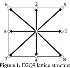
velocity directions and magnitudes and varying particle mass are reduced (in the simple 2-D model we focus on here) to 8 directions, 3 magnitudes, and a single particle mass. Figure 1 shows the cartesian lattice and the
velocities ea where a = 0, 1, …, 8 is a direction index
and e0 =0 denotes particles at rest. This model is known
as D2Q9 as it is 2 dimensional and contains 9 velocities. This LBM classification scheme was proposed by Qian et al. [2] and is in widespread use. Because particle mass is uniform (1 mass unit or mu in the simplest approach), these microscopic velocities and momenta are always effectively equivalent. The lattice unit (lu) is the fundamental measure of length in the LBM models and time steps (ts) are the time unit.
Figure 1. D2Q9 lattice structure
This problems cause that in some cases MRT2 model is
going to be considered. Although this method increases the stability and limitation of the solution domain but
simplicity of SRT3 is the reason to more usage of this
model.
Lid driven cavity flows are important in many industrial processing applications such as short-dwell and flexible blade coaters [7]. They also provide a model for understanding more complex flows with closed recirculation regions, such as flow over a slit, contraction flows and roll coating flows. Hence, the lid driven cavity flow is most probably one of the most studied fluid problem in computational fluid dynamics field. Due to the simplicity of the cavity geometry, applying a numerical method on this flow problem in terms of coding is quite easy and straight forward. Despite its simple geometry, the driven cavity flow retains a rich fluid flow physics manifested by multiple counter rotating recirculating regions on the corners of the cavity depending on the Reynolds number. Solution of the cavity flow has been studied by many scholars. Hou et al. [8] and Guo et al. [9] have studied cavity flow by LBGK model. Ghia [10] studied this problem by MRT model which in this model collision term in generally is different with LBGK. Etroke et al. [11] completely studied cavity flow problem in high Reynolds numbers with stream function and vorticity formulation method. Taneda investigated the effect of aspect ratio on the laminar regime experimentally [12], and results were verified numerically by Shen and Floryan [13]. By increasing the cavity depth, bottom corner vortices begin to grow and finally they merge and make another primary vortex. With further increases in cavity depth, two another bottom vortexes are created. This process continues as the cavity depth increases. Patil et al. [14] has simulated the cavity flow with LBGK model in different Reynolds number ranges from 50 until 3200, and different aspect ratios between K=1 and K=4. Their conclusions were Compatible with Taneda and Chen works results. Few studies have conducted in cavity flow problem with Reynolds number more than 3200 and aspect ratio beyond 1. Lin
2Multiple-Relaxation-Time 3Single-Relaxation-Time
et al. [15] simulated the deep lid driven cavity flow in Reynolds numbers between 100 and 7500 and aspect ratios K=1, 1.5, 4. They used MRT model and compared results with pervious works. In this paper, LBGK model with a proper boundary condition in inlet side, is used for deep lid driven cavity flow simulation in Reynolds number ranges between 100 and 5000. It is also used for aspect ratios equal with 1, 1.5 and 4, which is not used before. Results are compared with latest results.
2. BOLTZMANN EQUATION WITH BGK4
APPROXIMATION
Lattice Boltzmann equation which is used in this paper is written as [1]:
i i
i
i x c t t t f x t
f ( + d , +d )- ( , ) =W (1)
where,fi is the distribution function for the particles
which have discrete velocities indicated byci. Right
hand side of the above equation includes the collision term and BGK approximation is used for evaluate this term by the following form:
i i eq i i i F f f d t + -= W (2)
In Equation (2), t is the relaxation time, eq
i
f is the
equilibrium distribution function and diF indicates the
external forces field. As introduced in [1], the
equilibrium distribution function, fieqis evaluated by:
] . 2 3 ) . ( 2 9 . 3 1 [ 2 2 4
2 cu c cu c uu
c f s s s i eq
i =rw + + - (3)
In Equation (3), uand rare macroscopic velocity and
density, respectively. wi andciquantities are weight
factors and discrete velocities which in D2Q9 lattice, they are equal to :
where, c=dx/dt. For simplicity we assume that 1
=
= t
x d
d .
Chapman–Enskog expansion shows that lattice
Boltzmann equation satisfies the continuity and momentum equations. With substituting Equation (2) in Equation (1), one obtains:
)] , ( ) , ( [ 1 ) , (
) , (
t x f t x f t x f
t t x f
eq i i
i i
-= +
t d
(6)
The above equation consists of two parts. One of them refers to streaming and the other one is related to collision. For streaming term, we can write:
) , ( ) ,
(x c t t t f x t t
fi + id +d = i +d (7)
Equation (7) yields quantities of fi for adjacent areas
after one moment and collision process is evaluated by Equation (6). It should be noted, that is not important which of operations (streaming or collision) is at first, because the sequence of them is only significant. Fluid viscosity is given by relaxation time and the lattice sound velocity, as the following form:
2
) 2 1
( - cs
= t
u (8)
where, cs=c/ 3 . For positive values of viscosity, it is
necessary that the relaxation time parameter,t be more
than 0.5. But stability conditions forces that this amount has to be enough larger than 0.5. Macroscopic velocity and density in each point will be calculated by the following equations:
å å
==
i i
eq i
i f
f
r (9)
å
=å
=i i
eq i c i
if c f
c u
r (10)
To implement the LBM, the written code would be
following an algorithm as Figure 2. In Figure 2, f*
stands for distribution function after streaming.
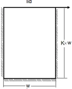
3. BOUNDARY CONDITIONS
In the current work, there are two kinds of boundary conditions. The first boundary condition is referred to the top of the cavity with uniform horizontal velocity (Figure 3). Second, boundary condition implies the static walls on the left, right and bottom of the cavity. On the static walls, no-slip boundary condition is applied and for this purpose bounce back rule is used. In this method to find the unknown distribution function after each streaming step, assume that distribution function is reflected in their moving direction. On the other hand, the orientation is fixed but direction is
inversed. Pseudo-code of this method on the bottom wall is shown as follows:
) 1 , ( ) 1 , (
) 1 , ( ) 1 , (
) 1 , ( ) 1 , (
8 6
4 2
7 5
x f x f
x f x f
x f x f
= = =
(11)
For the inlet boundary condition there are several suggestion such as Chen et al. [16], Zou et al. [3]. By these methods problem is easily solved when the aspect ratio K=1, but by increasing the cavity depth, using the above methods cause the slow convergence. To improve this defect in this paper we will use the method which is offered by Hou et al. [7]. Hou proposed substitution of the equilibrium distribution function to distribution function in this way:
Nx i Ny x f Ny x
fi( , )= ieq( , ), =1, (12)
where, Ny, represents the inlet side cavity.
Figure 2. Problem solving flowchart
4. NUMERICAL RESULTS
Now, the numerical solutions in case of different Reynolds numbers and aspect ratios in lid-driven cavity flow will be shown. In this problem, the dimensionless
cavity Reynolds number is defined as Re=U0Ny/u,
where U0 is uniform velocity which is on the top of the
cavity, Ny is the width of the cavity andu is the
kinematic viscosity of fluid. Aspect ratio is
characterized by Kand its value is equal with 1, 1.5 and
4, respectively. In fixed K number, we change the Re from 100 up to 5000. Lin et al. [15] showed that mesh sizes have less effect on solutions accuracies especially
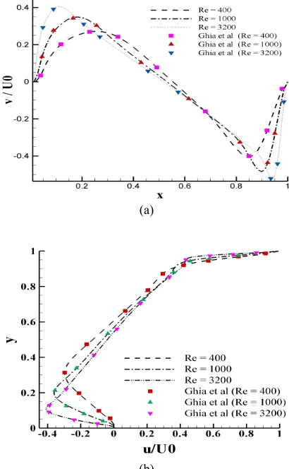
when the mesh sizes are greater than129´129. To verify
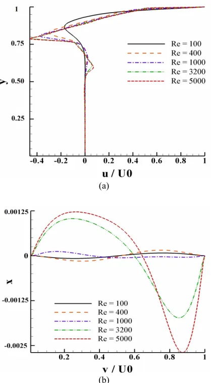
the written program code, the comparisons of predicted (a) horizontal and (b) vertical velocity with Ghia et al. [10] at different Reynolds number of aspect ratio K =1 are plotted in Figure.4 . For more precision, the location of primary vortex and two bottom secondary vortices of
K=1 are shown in Table 1 with solutions of [10, 15, 17].
(a)
(b)
Figure 4. Comparisons of predicted (a) horizontal and (b)
vertical velocity with Ghia et al. [10] at different Reynolds number-aspect ratio K =1
Figure 5. Streamline distributions at different Reynolds
number-aspect ratio K =1.
Structural changes in the vortex at different
Reynolds numbers of K=1 are shown in Figure 5. It is
clear that by increasing the Re, two bottom vortices are
slowlygrowing and when Re is becoming greater than
3200 another small vortex on the left top of the cavity is starting to grow. It can be clearly observed that the center of the primary vortex descends in tandem with the increase of the Reynolds number and remains constant beyond Reynolds number 3200. To investigate the effect of cavity depth on flow structure, we will study the case of K=1.5.
Horizontal and vertical velocity at different Reynolds number at K=1.5 are shown in Figure 6. This figure presents the predicted horizontal and vertical
velocities along x = 0.5 and y = 0.75, respectively. The
appearance of the second primary vortex can be observed from Figure 6a, where forward velocity is
present at location for y < 0.2. With increasing depth of
the cavity, the vortices in the lower corners are growing. As the Reynolds number is increasing these vortices merge and create second primary vortex (Figure 7). As the Reynolds number increases further, another two corner vortices would emerge. As we see, this event (merger of corner vortices) did not happen in the previous case when K=1. Comparing the detail results of the present work with Patil et al. [14], Pantil [17] and Lin et al. [15] are reported in Table 2.
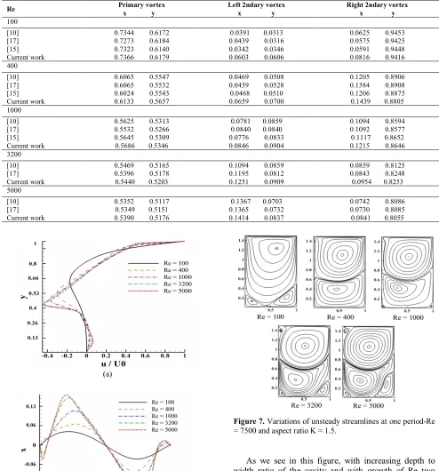
Figure 8, showing the predicted horizontal and
vertical velocities along x = 0.5 and y = 2, respectively.
It can be seen that below y = 2, the strength of the
vortex is rather week, reflected by the low level of
TABLE 1. Comparisons of the locations of the vortices at different Reynolds numbers with Ghia et al. [10], Pandit [17] and Lin et al. [15] – aspect ratio K =1
Right 2ndary vortex x y Left 2ndary vortex
x y Primary vortex
x y Re
100
0.0625 0.9453 0.0575 0.9425 0.0591 0.9448 0.0816 0.9416 0.0391 0.0313
0.0439 0.0316 0.0342 0.0346 0.0603 0.0606 0.7344 0.6172
0.7273 0.6184 0.7323 0.6140 0.7366 0.6179 [10]
[17] [15] Current work 400
0.1205 0.8906 0.1384 0.8908 0.1206 0.8875 0.1439 0.8805 0.0469 0.0508
0.0439 0.0528 0.0468 0.0510 0.0659 0.0700 0.6065 0.5547
0.6065 0.5532 0.6024 0.5543 0.6133 0.5657 [10]
[17] [15] Current work 1000
0.1094 0.8594 0.1092 0.8577 0.1117 0.8652 0.1215 0.8646 0.0781 0.0859
0.0840 0.0840 0.0776 0.0833 0.0846 0.0904 0.5625 0.5313
0.5532 0.5266 0.5645 0.5309 0.5686 0.5346 [10]
[17] [15] Current work 3200
0.0859 0.8125 0.0843 0.8248 0.0954 0.8253 0.1094 0.0859
0.1195 0.0812 0.1251 0.0909 0.5469 0.5165
0.5396 0.5178 0.5440 0.5203 [10]
[17] Current work 5000
0.0742 0.8086 0.0730 0.8085 0.0841 0.8055 0.1367 0.0703
0.1365 0.0732 0.1414 0.0837 0.5352 0.5117
0.5349 0.5151 0.5390 0.5176 [10]
[17] Current work
(a)
(b)
Figure 6. Predicted (a) horizontal and (b) vertical velocity at
different Reynolds number, K=1.5
Figure 7. Variations of unsteady streamlines at one period-Re
= 7500 and aspect ratio K = 1.5.
(a)
(b)
Figure 8. Predicted (a) horizontal and(b) vertical velocity at
different Reynolds number-aspect ratio K=4
TABLE 2. Comparisons of the locations of the vortices at
different Reynolds numbers with Patil et al. [14] and Pandit [17] – aspect ratio K = 1.5
2nd primary vortex x y 1st primary vortex
x y
Re 400
0.3906 0.4453 0.3950 0.4205 0.3825 0.4259 0.3949 0.4468 1.1172 0.5625
1.1241 0.5399 1.1030 0.5522 1.1093 0.5596 [14]
[17] [15] Current work 1000
0.4179 0.3007 0.3950 0.3439 0.4135 0.2960 0.4285 0.3111 1.0820 0.5352
1.0851 0.5399 1.0783 0.5293 1.0840 0.5346 [14]
[17] [15] Current work 3200
0.3632 0.3320 0.3560 0.3293 0.3692 0.3394 1.0703 0.5195
1.0668 0.5175 1.0718 0.5208 [14]
[15] Current work 5000
0.3504 0.3322 0.3622 0.3411 1.0658 0.5151
1.0684 0.5178 [15]
Current work
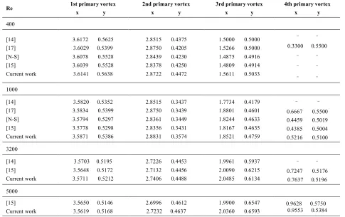
The results of his work have been inconsistent with [17], [15] and the present paper. For further verification, results of the NS calculations at Reynolds numbers 400 and 1000 are given by Lin et al. In addition, results at Reynolds numbers 3200 and 5000 are compatible with the results of Lin et al. and Patil. Comparisons of the locations of the primary vortices at different Reynolds numbers with Patil et al. [14], Pandit [17],Lin et al. [15]
and Navier–Stokes solutions are presented in Table 3.
Note that when the Reynolds number equals with 400
and K=1, no 4th primary vortex is reported, which is in
agreement with Patil et al. and Lin et al. works.
Consider the results reported by Pandit et al. predict 4th
primary vortex in this case, that may arise from their numerical errors.
TABLE 3. Comparisons of the locations of the primary vortices at different Reynolds numbers with Patil et al. [14], Pandit [17], Lin et al. [15] and Navier–Stokes solutions – aspect ratio K =4.
4th primary vortex x y 3rd primary vortex
x y 2nd primary vortex
x y 1st primary vortex
x y
Re
400
-0.3300 0.5500
-1.5000 0.5000 1.5266 0.5000 1.4875 0.4916 1.4809 0.4914 1.5611 0.5033 2.8515 0.4375
2.8750 0.4205 2.8439 0.4230 2.8378 0.4250 2.8722 0.4472 3.6172 0.5625
3.6029 0.5399 3.6078 0.5528 3.6039 0.5528 3.6141 0.5638 [14]
[17] [N-S] [15] Current work
1000
-0.6667 0.5500 0.4459 0.5019 0.4385 0.5004 0.5216 0.5100 1.7734 0.4179
1.8801 0.4601 1.8244 0.4633 1.8167 0.4635 1.8521 0.4759 2.8515 0.3437
2.8750 0.3439 2.8361 0.3449 2.8356 0.3431 2.8831 0.3574 3.5820 0.5352
3.5834 0.5399 3.5794 0.5297 3.5778 0.5298 3.5871 0.5386 [14]
[17] [N-S] [15] Current work
3200
-0.7247 0.5176 0.7637 0.5196 1.9961 0.5937
2.0090 0.6215 2.0485 0.6134 2.7226 0.4453
2.7132 0.4456 2.7406 0.4488 3.5703 0.5195
3.5648 0.5172 3.5711 0.5212 [14]
[15] Current work
5000
0.9628 0.5750
0.9553 0.5384 1.9900 0.6547
2.0360 0.6593 2.6996 0.4612
2.7232 0.4637 3.5650 0.5146
3.5619 0.5168 [15]
Current work
5. CONCLUSION
In this paper, LBGK model is used to simulate two dimensional lid-driven cavity flow at different Reynolds numbers between 100 and 5000 and three aspect ratios, K=1, 1.5 and 4 which is not used before. Implementation of appropriate boundary conditions is discussed in order to achieve reasonable convergence. It is reported that bounce back boundary condition in static walls with equilibrium distribution function in the inlet boundaries will tend to appropriate convergence. Flow structures were studied in details and good agreements were obtained. For a square cavity, results show that with increasing the Reynolds number, bottom
corner vortices will grow but they won’t merge together.
Moreover, the merger of the bottom corner vortices into a primary vortex and creation of other secondary vortices was shown in the cases which the aspect ratios are bigger than one. The merger of the bottom corner vortices into a primary vortex, and the reemergence of the corner vortices as the Reynolds number increases are more
evident for the deep cavity flows. For K=4 cavity flow,
four primary vortices are predicted by LBGK model for Reynolds number beyond 1000, which was not predicted by previous LBGK models, and results were
verified by Lin et al.
6. REFERENCES
[1-17]
1. Chen, S. and Doolen, G. D., "Lattice boltzmann method for fluid flows", Annual review of fluid mechanics, Vol. 30, No. 1, (1998), 329-364.
2. Qian, Y., d'Humières, D. and Lallemand, P., "Lattice bgk models for navier-stokes equation", EPL (Europhysics Letters), Vol. 17, No. 6, (1992), 479.
3. Zou, Q. and He, X., "On pressure and velocity boundary conditions for the lattice boltzmann bgk model", Physics of Fluids, Vol. 9, No., (1997), 1591.
4. Niu, X., Shu, C. and Chew, Y., "A thermal lattice boltzmann model with diffuse scattering boundary condition for micro thermal flows", Computers & Fluids, Vol. 36, No. 2, (2007), 273-281.
5. Ho, C. F., Chang, C., Lin, K. H. and Lin, C. A., "Consistent boundary conditions for 2d and 3d laminar lattice boltzmann simulations", CMES-Computer Modeling in Engineering & Science, Vol. 44, (2009), 137-155.
6. Liu, C.-H., Lin, K.-H., Mai, H.-C. and Lin, C.-A., "Thermal boundary conditions for thermal lattice boltzmann simulations",
Computers & Mathematics with Applications, Vol. 59, No. 7, (2010), 2178-2193.
7. Aidun, C. K., Triantafillopoulos, N. and Benson, J., "Global stability of a lid‐driven cavity with throughflow: Flow visualization studies", Physics of Fluids A: Fluid Dynamics, Vol. 3, (1991), 2081.
Journal of Computational Physics, Vol. 118, No. 2, (1995), 329-347.
9. Guo, Z., Shi, B. and Wang, N., "Lattice bgk model for incompressible navier–stokes equation", Journal of Computational Physics, Vol. 165, No. 1, (2000), 288-306. 10. Ghia, U., Ghia, K. N. and Shin, C. T., "High-resolutions for
incompressible flow using the navier-tokes equations and a multigrid method", Journal of Computational Physics, Vol. 48, (1982), 387-411.
11. Erturk, E., Corke, T. C. and Gökçöl, C., "Numerical solutions of 2‐d steady incompressible driven cavity flow at high reynolds numbers", International Journal for Numerical Methods in Fluids, Vol. 48, No. 7, (2005), 747-774.
12. Taneda, S., "Visualization of separating stokes flows", Journal of the Physical Society of Japan, Vol. 46, No. 6, (1979), 1935-1942.
13. Shen, C. and Floryan, J., "Low reynolds number flow over cavities", Physics of Fluids, Vol. 28, (1985), 3191.
14. Patil, D., Lakshmisha, K. and Rogg, B., "Lattice boltzmann simulation of lid-driven flow in deep cavities", Computers & Fluids, Vol. 35, No. 10, (2006), 1116-1125.
15. Lin, L.-S., Chen, Y.-C. and Lin, C.-A., "Multi relaxation time lattice boltzmann simulations of deep lid driven cavity flows at different aspect ratios", Computers & Fluids, Vol. 45, No. 1, (2011), 233-240.
16. Chen, S., Martinez, D. and Mei, R., "On boundary conditions in lattice boltzmann methods", Physics of Fluids, Vol. 8, (1996), 2527.
17. Pandit, S. K., "On the use of compact streamfunction-velocity formulation of1stready navier-stokes equations on geometries beyond rectangular", Journal of Scientific Computing, Vol. 36, No. 2, (2008), 219-242.
Simulation of Lid Driven Cavity Flow at Different Aspect Ratios Using Single
Relaxation Time Lattice Boltzmann Method
M. Taghiloua, M. H. Rahimianb
a Faculty of Mechanical Engineering, University of Tabriz, Tabriz, Iran
b School of Mechanical Engineering, College of Engineering University of Tehran, Tehran, Iran
P A P E R I N F O
Paper history:
Received 24 April 2013
Received in revised form 31 May 2013 Accepted 20 June 2013
Keywords:
Cavity Flow Lattice Boltzmann Aspect Ratio Vortex Integration
هﺪﯿﮑﭼ
ﻪﮑﺒﺷ ﻦﻣﺰﺘﻟﻮﺑ لﺪﻣ ﻪﻟﺎﻘﻣ ﻦﯾا رد دﺮﻔﻨﻣ يزﺎﺳ ﺎﻫرنﺎﻣز ﺎﺑ يا
)
SRT
(
رد هﺮﻔﺣ ﻞﺧاد رد نﺎﯾﺮﺟ يزﺎﺳ ﻪﯿﺒﺷ ياﺮﺑ ،
هدوﺪﺤﻣردﻒﻠﺘﺨﻣيﺎﻫزﺪﻟﻮﻨﯾر
5000 -100
يﺮﻈﻨﻣﺖﺒﺴﻧﻪﺳردو
K=1
،
K=1.5
و
K=4
ﺖﺳاهﺪﺷﻪﺘﻓﺮﮔرﺎﮐﻪﺑ
.
ﻪﺑ
لﺪﻣرديزﺎﺳﺎﻫرنﺎﻣزراﺪﻘﻣ بﺎﺨﺘﻧاردﺖﯾدوﺪﺤﻣدﻮﺟوﺖﻠﻋ
SRT
ﺎﺑشورﻦﯾا زاهدﺎﻔﺘﺳاﺎﺑنﺎﯾﺮﺟيزﺎﺳﻪﯿﺒﺷ،
ﺖﯾدوﺪﺤﻣﻦﯾاﻪﮐدﻮﺷﯽﻣﻪﺟاﻮﻣيدﺎﯾزيﺎﻫﺖﯾدوﺪﺤﻣ ﺪﯿﺸﺨﺑدﻮﺒﻬﺑﺐﺳﺎﻨﻣيزﺮﻣطﺮﺷلﺎﻤﻋاﺎﺑناﻮﺗﯽﻣارﺎﻫ
.
ياﺮﺑ
هراﻮﯾدردشﺰﻐﻟمﺪﻋيزﺮﻣطﺮﺷلﺎﻤﻋا ﺑﺖﺸﮔزﺎﺑطﺮﺷزاﺎﻫ
ﻂﺳﻮﺗهﺪﺷﻪﺋارايزﺮﻣطﺮﺷزايدوروﺖﻤﺴﻗردو ﺐﻘﻋﻪ
ﺖﺳاهﺪﺷهدﺎﻔﺘﺳاﻮﻫيﺎﻗآ
.
ﯽﻣنﺎﺸﻧﯽﻌﺑﺮﻣهﺮﻔﺣﮏﯾياﺮﺑﺞﯾﺎﺘﻧ ﻪﺑادﺮﮔزﺪﻟﻮﻨﯾردﺪﻋﺶﯾاﺰﻓاﺎﺑﻪﮐﺪﻨﻫد
ودرددﻮﺟﻮﻣيﺎﻫ
ﺪﻧﻮﺷﯽﻤﻧﺐﯿﮐﺮﺗﺮﮕﯾﺪﮑﯾﺎﺑﺎﻣادﻮﻤﻧﺪﻨﻫاﻮﺧﺪﺷرﻦﯿﯾﺎﭘﻪﺷﻮﮔ
.
هﺮﻔﺣﻦﯿﯾﺎﭘردﯽﻣودﻪﺑادﺮﮔدﺎﺠﯾاﻦﯿﻨﭽﻤﻫ ﻖﻤﻋﺶﯾاﺰﻓاﺎﺑ
ﺖﺳاهﺪﺷهدادنﺎﺸﻧﯽﺑﻮﺧﻪﺑهﺮﻔﺣ
.
راﺪﻘﻣﻪﺑيﺮﻈﻨﻣﺖﺒﺴﻧﻪﮐﯽﺘﻟﺎﺣرد
4
ﯽﻣ هﺮﻔﺣﻞﺧادردﯽﻠﺻاﻪﺑادﺮﮔرﺎﻬﭼﺪﺳر
ﯽﻣﺖﺳﺪﺑ يﺎﻫلﺪﻣﻪﮐﺪﯾآ
SRT
ﺪﻧاﻪﺘﺷاﺪﻧارﺖﻟﺎﺣﻦﯾايزﺎﺳﻪﯿﺒﺷناﻮﺗﻦﯿﺸﯿﭘ
.
ﺎﺑﻪﻟﺎﻘﻣﻦﯾاردهﺪﻣآﺖﺳﺪﺑيدﺪﻋﺞﯾﺎﺘﻧ
ﺴﯾﺎﻘﻣﺰﯿﻧﻪﺘﺷﺬﮔتﺎﻘﯿﻘﺤﺗﺞﯾﺎﺘﻧ ﺖﺳاهﺪﺷﻪ
.