Large Deflection Analysis of Compliant Beams of Variable Thickness and Non-Homogenous Material under Combined Load and Multiple Boundary Conditions

International Journal of Engineering

Large Deflection Analysis of Compliant Beams of Variable Thickness and

Non-homogenous Material under Combined Load and Multiple Boundary Conditions

A. Khavvaji, M. H. Pashaei*_{, M. Dardel, R. A. Alashti}

Babol Noshirvani University of Technology, Department of Mechanical Engineering, P.O. Box 484, Babol, Iran

P A P E R I N F O

Paper history:

Received 14 July 2012

Received in revised form 11 October 2012 Accepted 18 October 2012

Keywords: Large Deflection Compliant Mechanisms Geometric Nonlinearity Multiple Shooting Method Quadratic Programming.

A B S T R A C T

This paper studies a new approach to analyze the large deflection behavior of prismatic and non-prismatic beams of non-homogenous material under combined load and multiple boundary conditions. The mathematical formulation has been derived which led to a set of six first-order ordinary differential equations. The geometrically nonlinear problem has been solved numerically using the multiple shooting method combined with a quadratic programming technique. The results obtained by presented method have been compared with the existing with less complex cases in the literature. The method may be applied to the design of compliant mechanisms, nonlinear springs or any related subject.

doi:10.5829/idosi.ije.2013.25.04c.10

1. INTRODUCTION1

Conventional mechanisms have been studied and extensively implemented in past centuries. The use of flexibility in structures and mechanisms was mostly avoided because of the difficulty in design and manufacturing. In recent decades, compliant mechanisms (CM) have become an important area in mechanical science which is rapidly developing due to dramatic improvement of technology, need for high precision, smal scale and low final cost. Compliant mechanisms are usually monolithic and transmit motion and forces by means of their flexible members. Therefore CMs’ members usually undergo large deflection without exceeding the yield stress of the material. The advantages of these mechanisms compared to traditional rigid-body mechanisms are due to the absence of rigid body kinematic joints. Some of the many advantages of these mechanisms includes lower degree of noise, backlash and lubrication as well as wear; resulting in structures with very low maintenance cost and high precision. Compliant mechanisms are widely used in product design [1–3], design for systems without assembly proccess[4], Micro

*_{Corresponding Author Email: [email protected] (M. H. Pashaei)}

Electro Mechanical Systems (MEMS) [5], nonlinear springs [6, 7], stages for precision engineering [8], statically balanced mechanisms [9, 10].

including unbounded Gauss-Newton Method and bounded Gauss-Newton Method [15]. An approximate power series solution using an incremental linearization approach in global coordinate model was implemented to investigate deformed shape of compliant mechanisms with large displacement and rotation [16].

In that work, the concentrated loads were applied to a compliant mechanism of initially curved members. The analytical homotopy analysis method (HAM) has been used to investigate the large deformation of a cantilever beam under point follower load at the free tip [17, 18]. An analytical analysis investigation on large deflection of cantilever beams subjected to end point load has also been studied using the Adomian decomposition method (ADM) [19] and direct nonlinear solution (DNS) [20]. A comparative review of different methods regarding computation time, implementation convenience and accuracy was reported in the literature [20]. Nonlinear elastic behavior of materials, makes the problems more complex. Large deflection of a linear viscoelastic slender cantilever beam subjected to a time dependent concentrated load at the free end has been investigated by Vaz and Caire [21]. Solano investigated exact solutions for the large deflection of a cantilever beam made of Ludwick type material under a concentrated loading at the free end as well as a uniformly distributed vertical load [22]. An initially curved partially compliant bi-stable mechanism was also studied by Tolou and Herder [10].

Most of the beams which have been investigated in the above mentioned studies are the classical type of compliant beams which were subjected to tip loads, while a few of them were subjected to distributed loads; with variable thickness or nonlinear materials [22, 23, 16]. In addition, Lee has carried out the Post-buckling analysis of uniform columns under combination of a uniformly distributed axial load and concentrated load at the free end [24] using Butcher's numerical integration procedure. Then Merli et al. have analyzed the nonlinear bending problem of a constant cross-section extensible beam with simply supported ends subjected to a uniformly distributed load [25].

In the above studies, the numerical integration was derived using a nonlinear Timoshenko beam and two different linearization schemes, namely, multistep transversal linearization (MTrL) and multi-step tangential linearization (MTnL).

In this article, the previous works have been extended by analyzing the large deflection of a variable thickness beam. The non-homogenous material under general loading cases consisting of concentrated end tip force, end tip moment, and distributed loading were also considered. Large deflections analysis of beam was carried out considering multiple boundary conditions including, clamped, simply supported, free and sliding. The mathematical formulation of this problem yields to a set of six first-order ordinary differential equations

consisting components of slope, moment, forces and positions of each point of the beam in global Cartesian coordinates. The shooting method has been used to solve the governing equations numerically. The two point boundary value problem (BVP) is transformed into an initial value problem (IVP). The solution starts by assuming an initial conditions and continues with integration of the equations using the Runge-Kutta algorithm [26].

By adjusting the assumed initial values using iterative methods, the terminal boundary conditions will be convergence to an acceptable degree of accuracy. This adjustment is implemented by minimization of errors in terminal boundary conditions using an optimization algorithm such as Newton’s or quasi-Newton’s method. This procedure has a simple formulation and high accuracy with extreme convergence speed [26]. Unlike the finite element method which requires fine meshing to increase the accuracy, this method does not depend on element size and correspondingly may reduce the computation time. Without loss of generality, the shear and axial deformations are assumed insignificant because of their small values compared to flexural deformation of slender beams. Several numerical examples are presented covering prismatic and non-prismatic cantilever beams subjected to a general loading consisting of moments, distributed loads and concentrated loads in vertical and horizontal directions. The beams are inextensible, linear elastic and initially straight with various boundary conditions at both ends.

This paper is organized as follows: the moment-curvature relationship and governing equation are first derived in section 2. 1. In section 2. 2, constraints and loading cases are introduced; section 2. 3 presents the shooting method as the numerical solver. The results are portrayed graphically and presented numerically in section 3 and compared with those of the numerical solution obtained from FEM. Discussion on obtained results are presented in section 4 and finally, section 5 represents the conclusions.

2. MATHEMATICAL MODEL

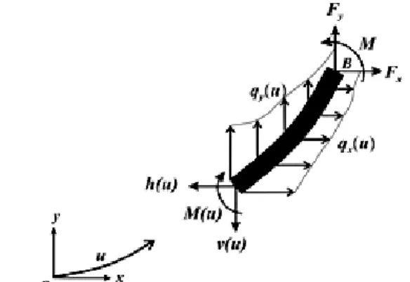
2. 1. Governing Equation Figure 2 shows the free body diagram of a compliant beam segment from point (

x

,

y

Figure 1. Non-prismatic compliant beam under generalized loading

Figure 2. Free body diagram of the compliant beam segment

Figure 3. Infinitesimal element in global coordinate system

Horizontal and vertical equilibrium force equations of this segment are:

(1) ( ) L ( )

H s =ò_SW_x s ds+F_x

(2)

( ) L ( )

V s =ò_SW s ds F_y + _y

Consider an infinitesimal element of length ds of the beam as shown in Figure 3.

Applying the moment equilibrium of the element yields:

(3)

( ) _{( ) ( ) 0}

dM s _{ds V s dx H s dy}

dS + - =

The link is characterized by a nondimensional arc length ]

1 , 0 [ Î

u along its neutral axis that is defined as u=s L . From Euler–Bernoulli law and the geometrical relationship of the infinitesimal element:

(4) )

( ) ( )

( u

du d L

u EI u

M = y

(5) ))

( ) ( cos( u u L

x du

d _{= y +h}

(6) ))

( ) ( sin( u u L

y du

d _{= y +h}

where Ψ and η are the angle of rotation and initial slope of the beam, respectively. As shown in Equation 4, both non-uniform moment of inertia, I(u), and non-homogenous Young’s modulus, E(u), can be incorporated. Substituting Equations (4), (5) and (6) into Equation (3), results in:

(7)

2

1

( ( ) ( )) ( ) cos( ( ) ( ))

( ) sin( ( ) ( )) 0

d

EI u u V u u u

du L

H u u u

y y h

y h

¢ + +

-+ =

The prime over a variable denotes the first derivative with respect to u.The detail of above derived equations are found in the literature [23].

Equations (1), (2), (5), (6) and (7) are the governing equations of the large deflection behavior of cantilever beams of non-uniform thickness and non-homogeneous material subjected to various types of loadings. In order to proceed solving the equations use the direct multiple shooting method, the beam is divided into N arbitrary subsegments by N-1 control points. In each subsegment, η, EI are constant and Wx,W are uniform. As the y number of control points increases, it can be shown the accuracy of the results increases.

On the other hand the computational procedure and consequently, the CPU time increased. Dividing the beam in the subsegments less than 10 (i.e N £10 ) is usually sufficient to determine the shape of a compliant beam.

Equations (1), (2), (5), (6), and (7) form a system of coupled first-order ordinary differential equations as follows:

(8) 2

( sin( ) cos( ))

cos( ) sin( )

( ) ( ) i i

Li _{H V}

i i i i i i i

EIi xi

q_i L_{i i i}

yi

Li i i

Hi

L Wxi i Vi

L Wyi i

y y

y y h y h

y h y h

¢ ¢

¢ + - +

¢ = = +

+

-ì ü

ì ü ï ï

ï ï ï ï

ï ï ï ï

ï ï ï ï

ï ï ï ï

í ý í ý

ï ï ï ï

ï ï ï ï

ï ï ï ï

ï ï ï ï

î þ

ï ï

î þ

Each set of governing Equation (8) can be applied to any sub segment. In each sub segment the non-dimensional parameter

u

(9)

0=u₀<u₁< <... _uN=1

The [ , ₁T T₂, ... T T] N

q=q q q is the vector of unknowns of the flexible beam. Equation (8) is a set of ordinary differential equations which can be solved numerically by algorithms such as “ode45” in MATLAB® _[29], using an initial guess for vector q. However, the problem of the beam is a BVP which is then treated as an IVP.

2. 2 Boundary Conditions Both ends of the beam are constrained, which can be expressed by constraint equations. The equations may be divided into four classes including force, position, moment and slope constraints depending on the joint type. The joints are also categorized in four types including clamped, simply supported, free and sliding. The joints along with the boundary conditions are shown in Table 1.

TABLE 1 . Boundary conditions and joint types

Force Position Moment Slope

Clamp NA* i

i x const y const = = ì í

î yi =0 NA

Simply

Support NA

x_i const y_i const

= = ìï í ïî EIi _Me i

Liy¢ = NA

Free i x

i y H F V F = = ì í î NA EIi Me i

Li y¢ = NA

Sliding

Along

x axis Hi=Fx yi=const EIi i Me Li y¢ = NA

Along

y axis Vi=Fy xi=const

EIi Me i

Li y¢ = NA *_{NA: not available and are to be determined during computation}

The bending moment and forces are normalized as

(10)

2 2 3

, , ,

(0) (0) (0)

3 ,

(0) 2 (0)

L L L

F_x F_x F_y F_y W_x W_x

EI EI EI

L L

W_y W_y M M

EI pEI

= = =

= =

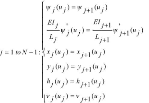
When a beam is divided into N subsegments, it has )

1 (

6´ N- continuity conditions at each control point as shown in Equation (11) for the forces, positions, moment and slope in each subsegment.

(11)

( ) ₁( )

1

' _{( )} ' _{( )} 1 1 ( ) ( )

1 1 : ₁

( ) ₁( )

( ) ₁( )

( ) ₁( )

u u

j j j j

EI

EI j j

u u

j j j j

L_j L_j

x u x u

j to N _{j j j j}

y u_{j j} y_j u_j

h u_{j j} h_j u_j

u u

j j j j

y y y y n n = ₊ + = ₊ + = = - ₊ = ₊ = ₊ = ₊ ì ï ï ï ï ï í ï ï ï ï ïî

From Equation (8), a beam has 6´ N differential equations, a number that must be equal to the number of constraint equations in order to be solved to obtain

N

´

6 unknowns. There are 6 constraints at both end points which are presented in Table 1. As a result, a beam with N sub segments has 6´ N constraint equations. So, the number of equations is equal to the number of boundary conditions. Constraint equations including boundary conditions and continuity equations lead to a vector of nonlinear algebraic equations:

(12) 0

)

(q =

F

2. 3. Multiplie Shooting Method The shooting method is an approach for solving a BVP by converting it to an IVP. The unknown initial values need to be assumed, and then the IVP to be solved to obtain the boundary values subsequently. If the obtained results are not equal to the predefined boundary conditions, an iterative approach such as Newton’s method will be applied. The initial guess will iteratively be changed until the boundary conditions on the other side are satisfied. Similar to solve nonlinear equations, the simple Shooting method has the following two major concerns in implementation:

· The solution is sensitive to the initial guess. For highly nonlinear or unstable problems, the initial guess has to be close enough to a solution. Wrong initial guesses may lead to singularities or cause the solutions not exist on bounds.

· Slow convergence of solutions. Solving nonlinear systems utilizes root finding techniques that typically make these methods converging at slower rate. Also the round off errors that emerge in each iteration may slow down the convergence rate of the solutions.

has been satisfied. Therefore, it is possible to approximate Equation (13) in each iteration (k th_{) by the} first-order function:

( ) ( ) ( )( )

F q @F q_k +J q_k q q- _k (13)

In this equation,

q

Jacobian matrix evaluated numerically at q_k using the finite difference method. Calculation of Jacobian matrix is very time consuming, hence, it the Quasi- Newton approach such as Broyden’s method [27] can be used to approximate the Jacobian matrix in each iteration. To find vector q by solving Equation (13), when the

|| ) ( ||

min F q become less than the tolerance ε the iteration will be terminated:

min || ( ) ||F q £e (14)

Next, the approximation Equation (15) is squared and expanded:

2

||J q b_k - _k || =(q J J qt t_{k k} -2b J q b b_{k k}t + _{k k}t ) (15)

To simplify the notation, the vectors _J(qk) and )

(q_k

F are defined as J_k and F_k, respectively. Where

k

b is a constant vector in each iteration and can be defined as follows:

b_k =J q_{k k}-F_k (16)

Since t _k

kb

b is a constant vector in each iteration, it can be eliminated from Equation (15). The remaining problem is to develop in the standard form of the quadratic programming problem (QP) which can be solved using various methods such as “fmincon” or “quadprog” in MATLAB®:

1

min( ) ; 2

t t

q Hq F q+ q_lb £ £q q_ub (17)

Solving the quadratic programming problem leads to find the vector q, that is the initial guess for the next step q_k+1. This iteration procedure will be repeated until Equation (14) is satisfied for a given ε.

3. RESULTS

Numerical examples will now be given to illustrate the validity of the present study and to investigate the force-deflection behavior of the beam under different boundary conditions. The nonlinear FEM result is obtained by the co-rotational procedure implemented in ANSYS® _{[30], in which the beam 3 element has been} used to perform large-displacement static analysis. The tolerance ε in all examples was set at 1e-8. The adopted dimensions in the numerical example are presented in Table 2.

TABLE 2. Geometrical properties adopted for the

numerical examples.

Length, L [mm] 50 In-plane thickness, h [mm] 0.4 out-plane thickness, b [mm] 6

Young’s modulus, E [GPa] 115 (titanium Ti-6 Al-2 V)[31]

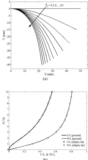
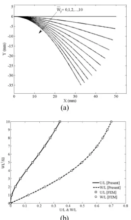
3. 1. Case I: Beam with Clamped-free Boundary Condition under End Point Force and Moment Figure 4(a) shows the trajectory position of an initially straight cantilever beam made up of linear elastic material under normalized end point concentrated load Fy(0 to 10 in –y direction). Figure 4(b) shows the non

dimensional loads versus non dimensional

displacements of end tip in x and y directions (U/L, W/L respectively). In Table 3 the results are compared with the elliptic integral solution [28].

(a)

(b)

TABLE 3. Comparison of present study results with those of the elliptic integral solution for case I under end point force

Fy

U L

W L

Ref [27] Present _Study Ref [27] Present _Study

1 0.05643 0.0564 0.30172 0.3017 2 0.16064 0.1606 0.49346 0.4935 3 0.25442 0.2544 0.60325 0.6033 4 0.32894 0.3289 0.66996 0.6700 5 0.38763 0.3876 0.71379 0.7138 6 0.43459 0.4346 0.74457 0.7446 7 0.47293 0.4729 0.76737 0.7674 8 0.50483 0.5048 0.78498 0.7850 9 0.53182 0.5318 0.79906 0.7991 10 0.55500 0.5550 0.81061 0.8106

(a)

(b)

Figure 5. Cantilever beam of case I under normalized end moments: (a) Trajectory position and (b) non dimensional moment versus x and y end tip displacements

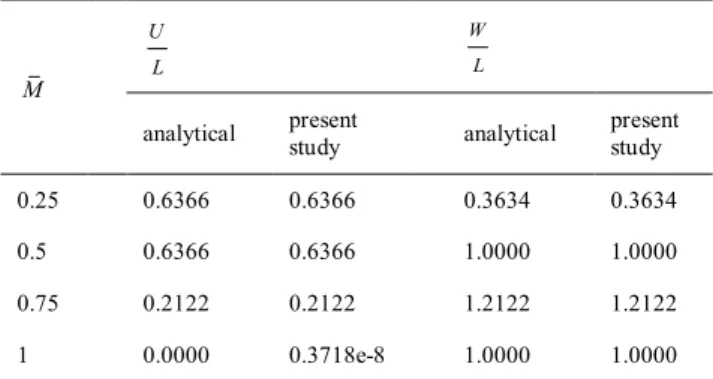
TABLE 4. Comparison of presented study with analytical method for case I under end moment

M

U L

W L

analytical present _study analytical present _study

0.25 0.6366 0.6366 0.3634 0.3634

0.5 0.6366 0.6366 1.0000 1.0000

0.75 0.2122 0.2122 1.2122 1.2122

1 0.0000 0.3718e-8 1.0000 1.0000

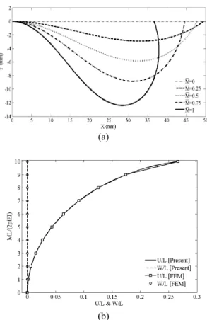
The trajectory position of a cantilever beam subjected to normalized end moment M (from 0 to 1) and four load steps are shown in Figure 5(a). Since all terms including forces, i.e. H(s) and V(s), in Equation (7) are zero, the

problem can have an analytical solution

(y( )u =2pM u´ ). Non dimensional loads versus non dimensional displacements and slopes are plotted in Fig. 5(b). In Table 4 a comparison of analytical solutions and the present numerical study is provided.

3. 2. Case II: Beam with Various Boundary Conditions under Uniform Distributed Loading

An inextensible beam with various boundary conditions such as clamped-free, clamped-sliding and simply supported-sliding under normalized uniformly distributed load W_y (0 to 10 in –y direction) has been investigated using the present method. The results are compared to those from a finite element solution. Since the load is uniform, the beam is considered without sub-segments (N=1).

Non dimensional force displacements of the beam for (a) clamped-free, (b) clamped-sliding and (c) simply support-sliding boundary conditions are shown in Figures 6, 7 and 8, respectively.

The results are compared to existing results in the previous studies [22]. As may be seen in Figures 6 there are not any difference between results of presented method and those of FEM, while there some differences as shown in Figures 7 and 8. That was due to the more complexity of supports of the beam.

(a)

(b)

Figure 6. Beam of case II with clamped-free boundary condition: (a) Trajectory position and (b) non dimensional load- displacement

(a)

(b)

Figure 7. Beam of case II with clamped-sliding boundary condition: (a) Trajectory position and (b) non dimensional load- displacement.

TABLE 5. Normalized displacements and slopes for (a) clamped-free, (b) clamped-sliding and (c) simply supported-sliding boundary conditions

y W

L U

L W

p y

2 1 0.0088 0.1235 0.0263 2 0.0331 0.2385 0.0512 3 0.0685 0.3396 0.0738 4 0.1099 0.4252 0.0937 5 0.1533 0.4959 0.1109 6 0.1963 0.5539 0.1258 7 0.2372 0.6015 0.1386 8 0.2756 0.6406 0.1496 9 0.3110 0.6731 0.1592 10 0.3436 0.7002 0.1675 (a) Clamp-Free

y W

L U

p y

2

1 0.2e-8 0.0022

2 0.0001 0.0045

3 0.0003 0.0068

4 0.0006 0.0090

5 0.0009 0.0112

6 0.0013 0.0135

7 0.0018 0.0157

8 0.0023 0.0179

9 0.0030 0.0201

10 0.0036 0.0222

(b) Clamp-Sliding

y

W

L U

p y 2

1 0.0004 0.0066

2 0.0017 0.0132

3 0.0037 0.0198

4 0.0066 0.0262

5 0.0102 0.0326

6 0.0144 0.0389

7 0.0193 0.0450

8 0.0248 0.0509

9 0.0307 0.0567

10 0.0371 0.0623

3. 3. Case III: Beam with Clamped-sliding Boundary Condition under End Point Moment The behavior of a beam with clamped-sliding boundary condition subjected to four normalized endpoint moment cases is depicted in Figure 9 (a). The results are compared to the finite element results. Figure 9 (b) shows the normalized endpoint slopes versus non dimensional arc length for each load case.

(a)

(b)

Figure 9. Beam of case III with clamped-sliding boundary condition: (a) Trajectory position and (b) non dimensional load- displacement.

3. 4. Case IV: Non-prismatic Beam with Clamped-sliding Boundary Condition under Non-uniform Distributed Loading In the final study a general case of research is presented. A non- prismatic beam with clamped-sliding boundary condition subjected to a ramp loading is shown in Figure 10 (a). Out of plane thickness is assumed to be uniform and equals to 1 mm (b=1mm), in plane thickness is varied from h1=0.6 mm at u=0 to h2=0.4 at u=1, respectively. The load w0 is equal to 800 N applied at u=0. Figure 10 illustrates the trajectory position and non-dimensional load-displacement of the beam with clamped-sliding boundary condition.

(a)

(b)

Figure 10. Non prismatic beam of case IV with clamp-sliding boundary condition under distributed ramp load: (a) Trajectory

position and (b) non dimensional load- displacement.

TABLE 6. comparison of convergence results for all case studies

Mean convergence iteration

computation time(s)

Accuracy

Case I (end force) 4 3.3910 1e-8 Case I (end moment) 1 2.3390 1e-8 Case II (Clamp-Free) 5 3.4940 1e-8 Case II

(Clamp-sliding) 5 4.1030 1e-8 Case II (simply

supported-sliding)

5 3.9620 1e-8

Case III 3 3.1180 1e-8 Case IV 6 4.8360 1e-8

Quasi- Newton algorithm and the iteration will be continued. Therefore, all of the computational time is spent to calculate the accurate value of the Jacobian matrix which is presented in all examples.

4. DISCUSSION

As data presented in Table 5, the computation time for all studied cases is found to be less than 5 seconds. The lowest computational recorded time corresponds to the Case I which is the cantilever beam under end point load, while the highest one (almost 2 times more) corresponds to Case IV which is the non-prismatic beam with clamped-sliding boundary condition under non-uniform distributed loading. As shown in this table, as the complexity of load case increases or the boundary condition changes towards cancelation of more degrees of freedoms, the computation time increases. This table also shows that an increase in number of sub-segments reduces the convergence rate and increases computational time. However, the solution still converges to a reasonably good accuracy as the number of load steps is increased. Reduction in number of load steps leads to divergence of results. This fact again shows that the nonlinear behavior depends on the loading history. Decreasing the value of ε increases the accuracy of results. However, it is less effective than increasing the number of sub-segments or load steps.

Some assumptions have been made to drive the governing Equation (9) including neglecting the bending effects and shear deformation. Nevertheless, the results are of good accuracy and agreed to those of FEM, as shown in Figures 4-9. It may be seen in Figures 4 and 6 that changes in the shape due to the distributed load is less as compared to the concentrated load. Also, as expected from Figures 7 and 8, the deflection will be increased (in the order of 10 percent) if one of boundary conditions is changed from clamped to simply supported. Figure 9 once gain validates the present approach as the slope at the clamped and simply supported ends matches with the boundary conditions. From Figure 10, it can be seen that the effect of the cross section on the deflection is also significant. This is due to the fact the area moment of inertia is more sensitive to in-plane thickness than out of plane thickness.

5. CONCLUSION

In this paper, large deflection of compliant beams of variable thickness made of non-homogenous material under combined load and multiple boundary conditions has been investigated. The problem was modeled mathematically, and the governing equations were

derived and solved numerically using a shooting method. The large deflection analysis of compliant beams in the form of generalized case e.g. combined load, variable thickness, non-homogenous material and multiple boundary conditions has been investigated. Several examples are presented and a comparison was performed with FEM results. The presented method features high degree of accuracy with a considerably good convergence rate and is capable of handling a wide range of cases. It was also found that the multiple shooting method is not sensitive to initial values. Unlike the other methods the quadratic programming problem does not need to calculate the inverse Jacobian matrix that may introduce singularities. Therefore, the presented study can extensively be used in design of compliant mechanisms as well as a comparative for accuracy assessment of other methods.

6. REFERENCES

1. L. L. Howell, Compliant Mechanisms, 2nd _{ed., JohnWiley &}

Sons, New York, USA, 2001.

2. F.K. Byers, A. Midha, “Design of a Compliant Gripper Mechanism”, Proceedings of the 2nd National Applied

Mechanisms & Robotics Conference. Cincinnati. Ohio. (1991)

XC.1-1–XC.1-12.

3. N.B. Crane, L.L. Howell, B.L. Weight, “Design and Testing of a Compliant Floating-Opposing-Arm (FOA) Centrifugal Clutch”,

Proceedings of DETC (2000) /MECH-14451.

4. G.K. Ananthasuresh, S. Kota, Designing Compliant Mechanisms,Journal of Mechanical Engineering, Vol. 117 (1995) 93–96.

5. N. Tolou, V. A. Henneken, J. L. Herder, “Statically balanced compliant micro mechanisms (SB-MEMS): Concepts and simulation”, proceeding of ASME DETC Biennial,

Mechanisms and Robotics Conference, Montréal, Québec,

Canada: ASME. 2010.

6. C.V. Jutte, S. Kota, “Design of Nonlinear Springs for Prescribed Load-Displacement Functions” ASMEJournal of Mechanical

Design, Vol. 130 No. (8) (2008) 081403.

7. C.V. Jutte, S. Kota, “Design of Single, Multiple, and Scaled Nonlinear springs for Prescribed Nonlinear response”, ASME

Journal of Mechanical Design Vol. 132 (2008) 011003.

8. Culpepper, M.L., Anderson, G. “Design of a low-cost nano-manipulator which utilizes a monolithic”, spatial compliant

mechanism. Precis. Eng. Vol. 28, (2004) 469–482

9. K. Hoetmer, J. L. Herder, C. J. Kim, “A Building Block Approach for the Design of Statically Balanced Compliant Mechanisms” ,ASME Conference Proceeding, IDETC/CIE2009 (2009)

10. N. Tolou and J.L. Herder, “Concept and modeling of a statically balanced compliant laparoscopic grasper”, Proceedings of DETC (2009) 86694.

11. Chainarong Athisakul, Somchai Chucheepsakul. “Effect of inclination on bending of variable-arc-length beams subjected to uniform self-weight”, Engineering Structures, Vol. 30 (2008) 902–908.

12. S. Srpcic, M. Saje. “Large deformations of thin curved plane beam of constant initial curvature”. International Journal of

13. B. W. Golley. “The solution of open and closed elasticas using intrinsic coordinate finite elements”, Computer Methods in

Applied Mechanics and Engineering, Vol. 146, (1997)

127–134.

14. C. M. Wang, S. Kitipornchai, “Shooting-optimization technique for large deflection analysis of structural members”,

Engineering Structures, Vol. 14, No 4,(1992) 231-240.

15. C. C. Lan, Generalized “Shooting Method for Analyzing Compliant Mechanisms With Curved Members”, Journal of

Mechanical Design, Vol. 128 (2006) 765–775.

16. C. C. Lan, “Analysis of large-displacement compliant mechanisms using an incremental linearization approach”,

Mechanism and Machine Theory Vol. 43 (2008) 641–658.

17. jiwanga, Jian-Kang Chena, Shijun Liaob. “An explicit solution of the large deformation of a cantilever beam under point load at the free tip”, Journal of Computational and Applied

Mathematics Vol. 212 (2008) 320 – 330.

18. A. Kimiaeifar, G. Domairry, S. R. Mohebpour, A. R. Sohouli, A. G. Davodi. “Analytical Solution for Large Deflections of a Cantilever Beam under Nonconservative Load Based on Homotopy Analysis Method”, Published online in Wiley

interscience. DOI 10.1002/num.20538.

19. N. Tolou and J. L. Herder. “A Semianalytical Approach to Large Deflections in Compliant Beams under Point Load”,

Mathematical Problems in Engineerin, Vol. 2009, Article ID

910896, 13 pages.

20. F. Morsch, N. Tolou, J.L. Herder, “comparison of methods for large deflection analysis of a cantilever beam under free end point load cases”, proceeding of ASME International Design Engineering Technical Conferences and Computers and

Information in Engineering Conference, San Diego, CA,

USA. 2009 Paper number DETC2009-86754.

21. M.A.Vaz, M.Caire. “On the large deflections of linear viscoelastic beams”,International Journal of Non-Linear

Mechanics, Vol. 45 (2010) 75–81.

22. E. Solano-Carrillo. “Semi-exact solutions for large deflections of cantilever beams of non-linear elastic behavior”, International

Journal of Non-Linear Mechanics, Vol. 44 (2009) 253 – 256.

23. M. Dado, S. Al-Sadder, “A new technique for large deflection analysis of non-prismatic cantilever beams”, Mechanics Research Communications Vol. 32 (2005) 692–703.

24. Kyungwoo Lee. “Post-buckling of uniform cantilever column under a combined load”, International Journal of Non-Linear

Mechanics Vol.36 (2001) 813-816.

25. R. Merli, C. Lázaro, S. Monleón, A. Domingo. “Comparison of two linearization schemes for the nonlinear bending problem of a beam pinned at both ends”, International Journal of Solids

and Structures Vol. 47 (2010) 865–874

26. H. B. Keller, “Numerical Methods for Two-Point Boundary-Value Problems”, Blaisdell Publishing, Waltham, MA, 2nd _ed.

1992.

27. C. G. Broyden .”A Class of Methods for Solving Nonlinear Simultaneous Equations”, Mathematics of Computation, Vol. 19 (1965), 577-593

28. K. Mattiasson, “Numerical results from large deflection beam and frame problems analyzed by means of elliptic integrals”,

International Journal for Numerical Methods in Engineering.

Vol.17 (1981) 145–153.

29. MATLAB Inc., MATLAB: “The Language of Technical Computing”, Version 7, the math works, 2005.

30. ANSYS Inc., Manual of ANSYS 11, ANSYS Inc., 2008.

31. Mark’s standard handbook for mechanical engineers, Mc Graw Hill, 10th _{ed. 1997.}

Large Deflection Analysis of Compliant Beams of Variable Thickness and

Non-homogenous Material under Combined Load and Multiple Boundary Conditions

A. Khavvaji, M. H. Pashaei, M. Dardel, R. A. Alashti

Babol Noshirvani University of Technology, Department of Mechanical Engineering, P.O. Box 484, Babol, Iran

P A P E R I N F O

Paper history:

Received 14 July 2012

Received in revised form 11 October 2012 Accepted 18 October 2012

Keywords: Large Deflection Compliant Mechanisms Geometric Nonlinearity Multiple Shooting Method Quadratic Programming.

هﺪﯿﮑﭼ

ﯽﻣيﺪﯾﺪﺟشورصﻮﺼﺧردﻖﯿﻘﺤﺗوﻪﻌﻟﺎﻄﻣﻪﺑﻪﻟﺎﻘﻣﻦﯾا

ﺮﯿﻏوﻦﮕﻤﻫيرﻮﺸﻨﻣﺮﯿﻏويرﻮﺸﻨﻣيﺎﻫﺮﯿﺗرﺎﺘﻓرﻪﮐدزادﺮﭘ

ﻤﻫ

ﯽﻣراﺮﻗﯽﺳرﺮﺑدرﻮﻣگرﺰﺑيﺎﻬﻧﺎﮑﻣﺮﯿﯿﻐﺗردارﻦﮕ

ﺪﻫد .

مﺎﺠﻧاﺐﮐﺮﻣيراﺬﮔزﺎﺑوتوﺎﻔﺘﻣيزﺮﻣﻂﯾاﺮﺷردﯽﺳرﺮﺑﻦﯾا

ﺖﺳاهﺪﺷ

.

زاﯽﻟﻮﻤﻌﻣﻞﯿﺴﻧاﺮﻔﯾدﻪﻟدﺎﻌﻣﺶﺷزاﻞﮑﺸﺘﻣتﻻدﺎﻌﻣهﺎﮕﺘﺳدﮏﯾﻞﯿﮑﺸﺗﻪﺑﺮﺠﻨﻣﺎﻫﺮﯿﺗﻦﯾاﯽﺿﺎﯾرلﺪﻣﻪﯿﻬﺗ

ﺪﯾدﺮﮔلواﻪﺒﺗﺮﻣ

.

دﺎﻔﺘﺳاﺎﺑﯽﺳﺪﻨﻫﯽﻄﺧﺮﯿﻏﻂﯾاﺮﺷ

ﻪﺑﺎﺗﺮﭘشورزاه

ﻪﻣﺎﻧﺮﺑوﻪﻧﺎﮔﺪﻨﭼيا

ﺪﯾدﺮﮔﻞﯿﻠﺤﺗﯽﻄﺧﺮﯿﻏيﺰﯾر

.

ﺪﯾدﺮﮔﻪﺴﯾﺎﻘﻣﻪﻨﯿﻣزﻦﯾاردهﺪﺷمﺎﺠﻧاتﺎﻔﯿﻘﺤﺗزادﻮﺟﻮﻣﺞﯾﺎﺘﻧﺎﺑقﻮﻓشورﺎﺑﻞﺣزاهﺪﻣآﺖﺳﺪﺑﺞﯾﺎﺘﻧ

.

نﺎﺸﻧﺞﯾﺎﺘﻧ

ﯽﻣ

ﯽﻣارشورﻦﯾا ﻪﮐﺪﻫد

فﺎﻄﻌﻧايﺎﻬﻣﺰﯿﻧﺎﮑﻣﯽﺣاﺮﻃياﺮﺑناﻮﺗ

ﻮﺿﻮﻣ ﺎﯾوﯽﻄﺧﺮﯿﻏيﺎﻫﺮﻨﻓ،ﺮﯾﺬﭘ

درﻮﻣﻂﺒﺗﺮﻣتﺎﻋ

دادراﺮﻗهدﺎﻔﺘﺳا

.