R E S E A R C H
Open Access
Robust dose-response curve estimation
applied to high content screening data analysis
Thuy Tuong Nguyen
2*?, Kyungmin Song
5?, Yury Tsoy
1, Jin Yeop Kim
1, Yong-Jun Kwon
3, Myungjoo Kang
5and Michael Adsetts Edberg Hansen
4*Abstract
Background and method: Successfully automated sigmoidal curve fitting is highly challenging when applied to large data sets. In this paper, we describe a robust algorithm for fitting sigmoid dose-response curves by estimating four parameters (floor, window, shift, and slope), together with the detection of outliers. We propose two
improvements over current methods for curve fitting. The first one is the detection of outliers which is performed during the initialization step with correspondent adjustments of the derivative and error estimation functions. The second aspect is the enhancement of the weighting quality of data points using mean calculation in Tukey?s biweight function.
Results and conclusion: Automatic curve fitting of 19,236 dose-response experiments shows that our proposed method outperforms the current fitting methods provided by MATLAB??snlinfitfunction and GraphPad?s Prism software.
Keywords: High content screening, Dose response curve, Curve fitting, Sigmoidal function, Weighting function, Outlier detection
Introduction
In recent years, the need for automatic data analysis has been amplified by the use of high content screening (HCS) [1] techniques. HCS (also known as phenotypic screening) is a great tool to identify small molecules that alter the dis-ease state of a cell based on measuring cellular phenotype. However, HCS always comes with an important caveat: there is little or no a priori information on the com-pound?s target. At the Institut Pasteur Korea (IP-K), we have applied high content screening using small interfer-ing RNA (siRNA) [2,3] at the genome scale. More recently, we applied the siRNA knockdown strategy for each gene from the genome and studied their effect on a given molecule producing a clear response on a cellular assay, to look for synergestic effects of a drug and target. Per-forming large-scale curve fitting for the biological activity of a large compound library can lead to a great number of
*Correspondence: [email protected]; [email protected]
?Equal contributors
2University of California, Davis, USA 4Videometer A/S, Horsholm, Denmark
Full list of author information is available at the end of the article
dose-response curves (DRCs) that require proper fitting. The overall process of fitting, rejecting outliers, and data point weighting of thousands to millions of curves can be a significant challenge. The quality of a dose-response curve fitting algorithm is a key element that should help in reducing false positive hits and increasing real compound hits.
Several solutions [4-9] have been proposed to perform curve fitting. One of the widely used nonlinear curve fit-ting algorithms was introduced by Levenberg-Marquardt (LM) [5,6]. This method belongs to the gradient-descent family. However, due to the sensitivity of the method, the data quality and the initial guess, the curve fitting algo-rithm is unfortunately susceptible to becoming trapped in local minimums. To obtain proper curve fitting results, there is a need for automatic outlier handling, usage of predefined initial curves, and adaptive weighting for data points [10,11]. All of these demands can, without doubt, be applicable to large sets of data. Nonlinear and non-iterative least square regression analysis was presented in [7] for robust logistic curve fitting with detection of possible outliers. This non-iterative algorithm was imple-mented in a microcomputer and assessed using different
biological and medical data. A review of popular fitting models using linear and nonlinear regression is given in [4]. The study serves as a practical guide to help researchers who are not statisticians understand statistical tools more clearly, especially dose-response curve fitting using nonlinear regression. This book also describes the robust fitting algorithm and the outlier detection mecha-nism used in the commercial software GraphPad Prism?. In [8], an automatic best-of-fit estimation procedure is introduced based on the Akaike information criterion. This best-of-fit model guarantees not only the estimation of the parameters with smallest sum-of-squares errors but also good prediction of the model.
Simulated data for DRC estimation was used in [9] to examine the performance of the proposed Grid algorithm. The peculiarity of the Grid algorithm is that it visits all the points in a grid of four curve parameters and searches for the point with the optimum sum-of-squares error. A coarse-to-fine grid model and a threshold-based outlier detection mechanism were used to make the algorithm more efficient. This paper also provided Java-based soft-ware together with a sample dataset for academic use. However, the software is applicable only when the mea-surements are taken without replicates (one data point at each concentration). Furthermore, various popular com-puter software and code packages have been presented for DRC fitting such as the DRC package in R [12], the
nlinfitfunction in MATLAB? [13], and the XLfit add-in for Microsoft? Excel? [14].
In this paper, robust fitting and automatic outlier detec-tion based on Tukey?s biweight funcdetec-tion are introduced. This method was developed to automate nonlinear fit-ting of thousands of DRCs performed in replicates, detect the outliers automatically, and initialize the fitting curves robustly.
Background and method Background
In drug discovery, analysis of the dose-response curve (DRC) is one of the most important tools for evaluat-ing the effect of a drug on a disease. The DRC can be used to plot the results of many types of assays; its X -axis corresponds to the concentrations of a drug (in log
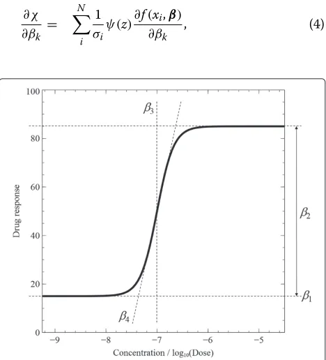
scale), and itsY-axis corresponds to the drug responses. The function of DRC can be varied with different number of parameters, but the four parameter model is the most common:
f(x,β)=β1+ β2
1+exp
? β3?x
β4
, (1)
where xis the dose or concentration of a data point;β represents the four parametersβ1, β2, β3, andβ4; β1is
the floor - the efficacy - which shows the biological activ-ity without a chemical compound;β2is the window - the
efficacy - which shows the maximum saturated activity at high concentration; β3is the shift - the potency - of the
DRC; andβ4is the slope - the kinetics. Figure 1 shows an
illustration of a response curve and its four parameters.
Basic computation of curve fitting
The goal of a curve fitting algorithm is to solve a statisti-cally optimized model that best fits the data set. Because the DRC function is nonlinear, an iterative method is con-sidered to optimize parameters. In this section, a basic viewpoint is presented to approach the proposed ideas in our method. First, let χ be the function of the fit-ting parameterβ which will be determined via function minimization:
χ(β)=
N
i ρ
yi? f(xi,β) σi
, (2)
whereρ(z)is an error estimation function of a single vari-ablez;σis a normalization value; andNis the number of data points. To minimize (2), the Newton method is used to search for zero crossing of the gradient:
βt+1=βt+D?1[?∇ χ(βt)] . (3) Hence, we need to find the gradient and the Hessian matrix Dof χ. The gradient ofχ with respect to β =
{β1,β2,β3,β4}is computed as ∂χ
∂βk = ? N
i 1 σiψ(
z)∂f(xi,β)
∂βk
, (4)
Figure 1A four-parameter dose-response curve.β1,β2,β3, andβ4
whereψ(z)is the derivative function ofρ(z)withz=(yi?
f(xi,β))/σi. The Hessian matrix is calculated using
∂2χ
∂βk∂βl = N i 1 σ2 i
ψ(z)∂f(xi,β)
∂βk
∂f(xi,β)
∂βl ?
1
σiψ( z)∂
2f(x
i,β)
∂βk∂βl
,
(5)
where the second derivative term is negligible compared to the first derivative. Let
akl = ∂
2χ
∂βk∂βl
andbk = ∂χ
∂βk
, (6)
where akl and bk are elements of matrices A and B, respectively; then instead of directly inverting the Hessian matrix, (3) can be rewritten as a set of linear equations:
4
l=1
aklδβl=bk, (7)
where δβl is changed at every iteration. Afterwards, to solve our fitting problem, we define
ρ(z)= 1
2z
2andψ(z)=z (8)
and obtainaklandbkusing least squares. The Levenberg-Marquardt (LM) method [5,6,15] solves (7) by defining a positive valueλto control the diagonal of the matrixA:
akk =akk(1+λ)andakl=akl (k=l). (9) The iteration steps of the LM method can be summa-rized as follows:
1. Evaluateχ(β)and define a modest value forλ, i.e., λ=0.001;
2. Solve (7) withA substituted byAin (9), and evaluate χ(β+δβ);
3. Ifχ(β+δβ)χ(β), increaseλby a factor of 10; else, decreaseλby a factor of 10 and updateβ←β+δβ; 4. Repeat steps 2 and 3 untilχ(β)converges, and the
returnβ.
Outlier detection
In most cases, it is difficult to estimate the parameters, either due to noise in the observations or because the experimental design might give rise to ambiguities in the parameters of the DRC. There is a need for an outlier detection mechanism to cope with noise before fitting curves. Figure 2 shows the effect of outliers in the data. There are eight different concentrations, five replicates at the first concentration, and three replicates at the remain-ing concentrations. It is likely to become noisy when the number of data points increases. Seven outliers (the solid arrows show these outliers in the figure) can change the fit of the curve dramatically. These seven points in the left figure have lower weights (outliers detected) than those in the right figure.
In our problem, we initialize the fitting parametersβo (disregarding outliers) by finding the best fitted curve using
ρ(z)= |z|andψ(z)=sign(z) (10)
instead of (8) which is used without outlier detection. Herein, we proposed (10) to reduce the impact of out-liers on the fitting results by considering absolute errors and sign-only derivatives. The key difference between (10) and (8) is that the derivative function: ψ(z) = sign(z)
results in? 1 (negative) or 1 (positive), which controls the gradient in the direction of having a higher number of negatives/positives, whereasψ(z)=zjudges the gradient based on the distance between the estimated and actual values. Therefore, (10) is able to disregard the points hav-ing a lower number of negatives/positives (see Figure 2, on the left), and (8) considers the points at far distances although these points are given low impact (see Figure 2, on the right). Levenberg-Marquardt and other conven-tional nonlinear curve fitting algorithms are based on derivative calculation, and the quality of their solutions notably depends on data quality (i.e., outliers) and the ini-tial guess. To have good fitting, outliers and the iniini-tial guess have to be manually detected and defined. Accord-ingly, these conventional algorithms are very difficult to automate and be made to yield good solutions in thou-sands of DRCs. Based on (10), outliers can be effectively weighted and a robust initial guess is automatically deter-mined at the beginning of the fitting process. The method of weighting data points is described in the next section.
Curve fitting with weighting function
Because all fitting parameters of the DRC are very impor-tant in understanding and assessing the effect of a chem-ical compound, it is essential to have a method that can estimate the curve in a robust way, i.e., coping with out-liers and assigning weights to data points. Initially all data points are supposed to have equal weights. However, this idea does not hold in many practical occasions. Therefore, a least squares method tends to give unequal weighting to data points, e.g., points that are closer to the fitted curve would have higher weighting values. In standard weight-ing, minimizing the fitting error (sum-of-squares) of the absolute vertical distances is not appropriate: points hav-ing high response values tend to have large deviations from the curve and so they contribute more to the sum-of-squares value. This weighting makes sense when the scattering of data is Gaussian and the standard devia-tion among replicates is approximately the same at each concentration.
Figure 2Influence of noise (the arrows show the outliers).Fitting on the left assigns low weights to the outliers to disregard them. Fitting on the right considers the outliers as useful data points and gives higher weights to these points.
considered, including relative weighting, Poisson weight-ing, and observed variability-based weighting [4]. Rela-tive weighting extends the idea of standard weighting by dividing the squared distance by the square of the corre-sponding response valueY; hence, the relative variability is consistent. Similarly, Poisson weighting and weighting by observed variability use different forms of dividing the response valueY. Indeed, minimizing the sum-of-squares might yield the best possible curve when all variations obey a Gaussian distribution (without considering how different the standard deviations at concentrations are). However, it is common for one data point to be far from the rest (caused by experimental mistakes); then, this point does not belong to the same Gaussian distribution as the remaining points and it contributes erroneous impact to the fitting. The Tukey biweight function [10] was intro-duced to reduce the effect of outliers. This weighting function considers large residuals and treats them with low weights, or even zero weights, so that they do not sway the fitting much. In this section, we present a modification of the Tukey function and apply it to our fitting.
Letω(r)be the weight of a data point that has a distance to the curve (residual) ofr; then, the biweight function is defined as
ω(r)= ⎧ ⎪ ⎨ ⎪ ⎩
1? r
c 22
, |r|<c
0, |r|>c
(11)
wherec = 6? median{ri}Ni=1
, 6 is a constant defined by Tukey, andNis the number of data points. This func-tion totally ignores or gives zero weighting to the points having residuals larger than six times the median resid-ual. Nevertheless, when the experimental data contains a great deal of noise (which usually occurs in biological
and medical assays), it can fall on a normal distribution easier than when they contain little noise. When our data approaches a normal distribution, the mean of residu-als is a better choice than the median of residuresidu-als (the median is useful if the data has extreme scores). In our case, based on experimental situations, we decided to use c = 6 ? mean{ri}Ni=1
= 6?r. Figure 3 shows the fitting results of using themedianandmean. The sum-of-squares error produced by using themeanis significantly better than by using themedian. Additionally, the curve fit by using themeanlooks more satisfactory than by using the median. Hence, the curve fitting algorithm with the modified Tukey biweight function can be summarized as follows:
1. Determine the distance from each data point to the curve, called the residual,r;
2. Calculate the weight of each point using (11) with?r
applied;
3. Assign new values to data points based on their weights.
In addition, other robust weighting functions can be considered such as Andrews, bisquare, Cauchy, Fair, Huber, logistic, Talwar, and Welsch [16]; however, the Tukey biweight function is known for its reliability, and it is generally recommended for robust optimization [17]. As we show further, the use of the Tukey biweight allows for improved DRC fitting results (see the Results section).
Robust univariate DRC estimation algorithm
Figure 3Results of using the median (left) and mean (right) calculations in the Tukey biweight function.
1. Find the initial curve with outlier detection by executing the LM algorithm and applying (10) instead of (8);
2. Based on the curve obtained, calculate the Tukey biweights of data points using (11);
3. Based on the obtained weights, execute the LM algorithm in the basic computation section and consider the weights of the data points.
4. Repeat steps 2 and 3 for a predefined number of iterations or until convergence.
Results
We have previously shown the ability to use the high content genome-wide silencing RNA (siRNA) screening approach on various cellular models [2,3]. The recent combination of drugs (at different concentrations) and siRNA (approximately 20,000) lead us to look for an automatic method to characterize a large number of dose-response curves obtained in those experimental condi-tions. Using MATLAB?, a curve fitting algorithm was implemented. We compared the fitting performance of our method to that of the nlinfitfunction in MAT-LAB? 2013a and the robust DRC fitting in GraphPad Prism? 6.0.
In our experiments, we used eight different concen-trations 0, 0.005, 0.01, 0.1, 0.4, 1, 5, and 20 ?M with five replicates at concentration 0 and three replicates at the other concentrations (26 data points in total). In this manuscript, the concentrations were plotted over theX -axis in log unit. The Y-axis shows the drug response, which was normalized in the range of 0 to 100. The ini-tial values of the parameters floor, window, shift, and slope used in the MATLAB?nlinfitfunction were defined based on values of data points as min(Y), max(Y) ?
min(Y), average(X), and ?0.6, respectively. By default, the algorithm uses bisquare (also known as Tukey biweight) as the robust weighting function. Indeed, MAT-LAB? applied the Levenberg-Marquardt (LM) algorithm and iterative reweighted least squares [16] for robust esti-mation. Accordingly, thenlinfitrepresents the case of using the traditional LM algorithm and Tukey biweight function where (8) and the median function are utilized. For our algorithm, we defined the initial DRC parameters in the first step (outlier detection) as in nlinfit, and then those parameters were corrected using the outlier detection step and used for the consequent fitting steps. According to step 4 of our DRC estimation algorithm, the number of iterations was predefined as 50, and the error tolerance for convergence was 0.0001.
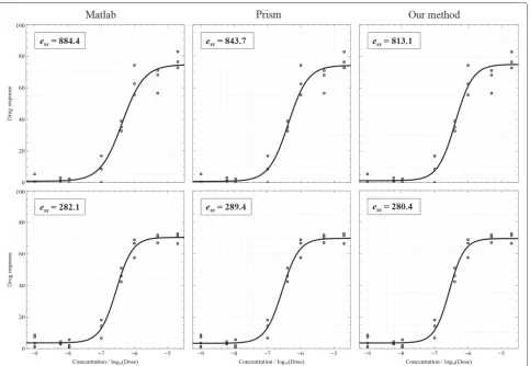
Figure 4 shows two examples of fitting when data points do not include outliers and the results of three fitting algo-rithms are acceptable. Curve fitting results were presented together with sum-of-squares errors (on the top-left cor-ner) which are calculated by taking the sum-of-squares of differences between the actualY and the estimatedY. Smaller errors indicate better results. The plotting results are shown from left to right: MATLAB?nlinfit, Prism?
Figure 6Two results of outliers and bad fitting.
robust fitting, and our method, respectively. Figure 5 illus-trates the cases of the presence of outliers. For points inside the interval from? 6.5 to? 5 (logunit), the varia-tion of measurements is high. In this figure, the first result of MATLAB?nlinfitdemonstrate an ambiguity of the shift parameter: thelog of IC50 should be shifted to the right to cross the mean point in the middle of the plot. The first plot of Prism? presents a poor DRC due to the high steep slope. Figure 6 displays the cases where out-liers appear and lead to bad fitting. Prism? was completely
unable to fit the first curve, but our method handled the data points very well. Additionally, the second plot of MATLAB?nlinfitshows an ambiguity of the shift parameter and a high steep slope.
In drug discovery and genome-wide data analysis, curve parameters, especially the shift, act as a crucial factor in determining the target candidates. Therefore, poor out-comes of the DRC fitting algorithm might greatly affect the analysis of the whole genome, which leads to dif-ficulty finding the targets. To evaluate the performance
Table 1 Averages and standard deviations of the normalized sum-of-squares errors calculated based on the fitting results of 19,236 curves
Slide Number of curves Matlab Prism Ours (median) Ours (mean)
? σ ? σ ? σ ? σ
1 3885 0.920 0.134 0.777 0.213 0.855 0.210 0.777 0.217
2 3887 0.907 0.117 0.852 0.154 0.943 0.134 0.817 0.165
3 3865 0.916 0.112 0.844 0.161 0.922 0.155 0.820 0.170
4 3875 0.946 0.105 0.793 0.198 0.841 0.202 0.777 0.207
5 3724 0.908 0.144 0.722 0.234 0.820 0.246 0.755 0.239
Average 0.919 0.122 0.798 0.192 0.876 0.189 0.789 0.200
of different DRC fitting algorithms on a large-scale, we assessed 19,236 curves which were obtained from five microarray slides. Table 1 shows fitting errors for the five slides with the corresponding number of curves 3885, 3887, 3865, 3875, and 3724 from each slide. Averages and standard deviations of the normalized sum-of-squares errors (the normalized error is calculated by dividing the actual error by the maximum one) were also included in this table with the comparison of the four methods. Herein, in addition to comparing our method (using mean calculation in the Tukey biweight function) to MATLAB? and Prism?, we also compared to our method, which uses the median for calculation of (11) to prove that the modi-fied Tukey biweight function can significantly improve the fitting. Our method mostly yielded the best average errors in all slides whereas MATLAB?nlinfitwas the worst. Prism? gave better results than the method using median calculation.
In summary, experimental comparisons show that our method (namely ?Ours (mean)? in the figure), which pro-poses automatic initialization of DRC parameters and modification of the Tukey biweight function (mean calcu-lation), yields a satisfactory fitting of curves. It provides more accurate fitting than MATLAB?nlinfit, where automatic initialization is not available and the default Tukey biweight function (median calculation) is used, by more than 14% in processing 19,236 curves. We also demonstrated that the method applying the automatic ini-tialization and the default Tukey function (namely ?Ours (median)?) did not yield results as good as those of ?Ours (mean)?. Moreover, the better performance of ?Ours (median)? than that of MATLAB?nlinfitimplies that the automatic initialization of DRC parameters meaning-fully improves the fitting process. Our method is supe-rior to GraphPad Prism? 6.0 by more than 1%. Although the error is slightly improved; we believe that, with the MATLAB? implementation provided, our approach is eas-ily automated and scalable to thousands of curves. It is able to process the entire genome data in less than two hours ? approximately 360 milliseconds for a curve (with a computer configuration using an Intel Core i7 3.47 GHz CPU).
Conclusion
We provide two improvements for the problem of DRC fitting: 1) increasing the accuracy of the initialization of DRC parameters with the use of outlier detection, and 2) improving the method of weighting for noisy data in the Tukey biweight function. Our method is adapted to the analysis of thousands of DRCs or more with the use of automatic outlier detection and initialization of curves. By experimentally comparing the results of our method to those calculated by thenlinfitfunction in MATLAB? 2013a and the robust DRC fitting in GraphPad Prism? 6.0,
we found that the proposed approach yielded a superior estimation of curves to that of MATLAB? and Prism?.
Competing interests
The authors declare that they have no competing interests.
Authors? contributions
Contributed idea: MAEH, KS, MK. Wrote manuscript: TTN, KS, YT. Implemented algorithm: TTN, KS. Did data analysis: TTN, MAEH, YJK. Designed and did biological experiments: JYK, YJK. All authors read and approved the final manuscript.
Acknowledgements
This work was supported by the National Research Foundation of Korea (NRF) grant funded by the Korea government (MEST) (No. 2012-00011),
Gyeonggi-do and KISTI. Kyungmin Song and Myungjoo Kang were supported by the National Research Foundation of Korea (NRF) grant funded by the Korea government (MEST) (2013-025173). The funders had no role in study design, data collection and analysis, decision to publish, or preparation of the manuscript.
Author details
1Institut Pasteur Korea, Seongnam-si, Gyeonggi-do, South Korea.2University of
California, Davis, USA.3Samsung Medical Center, Seoul, South Korea. 4Videometer A/S, Horsholm, Denmark.5Seoul National University, Seoul,
South Korea.
Received: 14 July 2014 Accepted: 14 November 2014
References
1. Joseph MZ:Applications of high content screening in life science research.Comb Chem High Throughput Screen2009,12(9):870?876. 2. Siqueira-Neto JL, Moon SH, Jang JY, Yang GS, Lee CB, Moon HK, Chatelain
E, Genovesio A, Cechetto J, Freitas-Junior LH:An image-based high-content screening assay for compounds targeting intracellular Leishmania donovaniamastigotes in human macrophages.PLOS Neglect Trop D2012,6(6):e1671.
3. Genovesio A, Kwon YJ, Windisch MP, Kim NY, Choi SY, Kim HC, Jung SY, Mammano F, Perrin V, Boese AS, Casartelli N, Schwartz O, Nehrbass U, Emans N:Automated genome-wide visual profiling of cellular proteins involved in HIV infection.J Biomol Screen2011,16(9):945?958. 4. Motulsky H, Christopoulos A:Fitting Models to Biological Data Using Linear
and Nonlinear Regression: a Practical Guide to Curve Fitting. New York, USA: Oxford University Press Inc.; 2004.
5. Levenberg K:A method for the solution of certain problems in least squares.Quart Applied Math1944,2:164?168.
6. Marquardt D:An algorithm for least-squares estimation of nonlinear parameters.SIAM J Applied Math1963,11(2):431?441.
7. Ayiomamitis A:Logistic curve fitting and parameter estimation using nonlinear noniterative least-squares regression analysis.Comput Biomed Res1986,19(2):142?150.
8. Rey D:Automatic best of fit estimation of dose response curve. Konferenz der SAS-Anwender in Forschung und Entwicklung 2007. [http://www.uni-ulm.de/ksfe2007]
9. Wang Y, Jadhav A, Southal N, Huang R, Nguyen DT:A Grid algorithm for high throughput fitting of dose-response curve data.Curr Chem Genomics2010,4:57?66.
10. Hoaglin D, Mosteller F, Tukey J:Understanding Robust and Exploratory Data Analysis. New York, USA: John Wiley and Sons Inc.; 1983.
11. Boyd Y, Vandenberghe L:Convex Optimization. Cambridge: Cambridge University Press; 2009.
12. Ritz C, Streibig JC:Bioassay analysis using R.J Stat Soft2005,12(5):1?22. 13. MathWorks Matlab 2013:nlinfit ? Nonlinear regression[http://www.
mathworks.com/help/stats/nlinfit.html]
15. Press WH, Teukolsky SA, Vetterling WT, Flannery BP:Numerical Recipes in C: the Art of Scientific Computing (3rd edition). New York, USA: Cambridge University Press; 2007.
16. Holland PW, Welsch RE:Robust regression using iteratively reweighted least-squares.Comm Stat Theor Meth1977,A6:813?827. 17. Maronna R, Martin RD, Yohai V:Robust Statistics ? Theory and Methods.
Chichester, England: Wiley; 2006.
doi:10.1186/s13029-014-0027-x
Cite this article as:Nguyenet al.:Robust dose-response curve estimation applied to high content screening data analysis.Source Code for Biology and Medicine20149:27.
Submit your next manuscript to BioMed Central and take full advantage of:
? Convenient online submission
? Thorough peer review
? No space constraints or color ?gure charges
? Immediate publication on acceptance
? Inclusion in PubMed, CAS, Scopus and Google Scholar
? Research which is freely available for redistribution