B R I E F R E P O R T S
Open Access
Easyworm: an open-source software tool to
determine the mechanical properties of worm-like
chains
Guillaume Lamour
1,2,3*, Julius B Kirkegaard
4, Hongbin Li
3, Tuomas PJ Knowles
4and Jörg Gsponer
1,3Abstract
Background:A growing spectrum of applications for natural and synthetic polymers, whether in industry or for biomedical research, demands for fast and universally applicable tools to determine the mechanical properties of very diverse polymers. To date, determining these properties is the privilege of a limited circle of biophysicists and engineers with appropriate technical skills.
Findings:Easyworm is a user-friendly software suite coded in MATLAB that simplifies the image analysis of individual polymeric chains and the extraction of the mechanical properties of these chains. Easyworm contains a comprehensive set of tools that, amongst others, allow the persistence length of single chains and the Young’s modulus of elasticity to be calculated in multiple ways from images of polymers obtained by a variety of techniques (e.g.atomic force
microscopy, electron, contrast-phase, or epifluorescence microscopy).
Conclusions:Easyworm thus provides a simple and efficient tool for specialists and non-specialists alike to solve a common problem in (bio)polymer science. Stand-alone executables and shell scripts are provided along with source code for further development.
Keywords:Matlab, GUI, Polymer, Worm-like chain model, Persistence length, Young’s modulus, AFM
Introduction
Although different approaches have been developed over the years to determine the nanomechanical properties of different biopolymers [1-3], it is mainly biophysicists and engineers with appropriate technical skills who have been able to use them. However, the growing number of technological applications for functional biopolymers such as modified cytoskeletal filaments or engineered DNA [4,5] asks for a fast and easy way to determine their mechanical properties that is also accessible to non-specialists. Here we present a new software tool, Easyworm [6], for the determination of the persistence length of polymer chains and derivation of their axial elastic modulus. This open-source software provides ac-curate measurements of the persistence length varied
over 6 orders of magnitude (from nm to mm ranges) and can be used by specialists and non-specialists alike.
Implementation
Easyworm consists of several graphical user interfaces (GUI) functioning as stand-alone applications for Micro-soft Windows or Linux operating systems. They require the appropriate MATLAB Compiler Runtime (MCR) version to be installed. Source code (.m) files along with GUIDE .fig files will also work under a MATLAB envir-onment. They can also be deployed as stand-alone exe-cutables or shell scripts, providing the MATLAB compiler toolbox is installed on the development ma-chine. MCR versions, executable files, shell scripts and the source code are freely available at http://www.chibi.ubc. ca/faculty/joerg-gsponer/gsponer-lab/software/easyworm. Detailed installation notes are provided on the same web-page. In addition, step-by-step instructions of how to use the software are provided in the Additional file 1 of this paper (Easyworm_SuppInfo.pdf).
* Correspondence:[email protected]
1
Centre for High-Throughput Biology, University of British Colombia, Vancouver, BC V6T 1Z4, Canada
2
Department of Chemistry, University of British Columbia, Vancouver, BC V6T 1Z1, Canada
Full list of author information is available at the end of the article
Methods overview
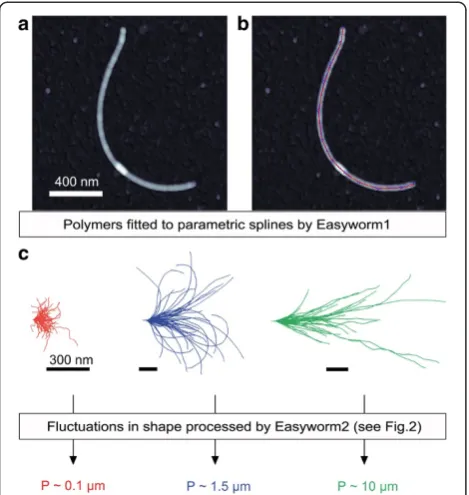
Easyworm is optimized for analyzing images of individ-ual polymer chains taken by atomic force microscopy (AFM; Figure 1) but can also be used for analyzing im-ages taken by other methods (e.g. electron microscopy,
epifluorescence, or simple contrast-phase optical micros-copy). Minimal user input is required in order to fit the contour of polymers to parametric splines (see Figure 1b) after uploading height maps in the first GUI,Easyworm1
(for detailed instructions see Additional file 1: Figure S1 and Note S1 in Easyworm_SuppInfo.pdf ). Then Easy-worm2 (second GUI; Additional file 1: Figure S2 and Note S2) is used to derive the mechanical properties from the data collected byEasyworm1.
Persistence length calculations
The persistence length P of a sample of individual poly-meric chains can be obtainedviathree distinct measures all derived from the worm-like chain model (WLC) for semi-flexible polymers. The choice of the measure to calculate P is highly dependent on the value of P with regard to the contour length of the polymer. For in-stance, P can be much higher (e.g. microtubules) or much lower (e.g. DNA) than the contour length. For quite flexible polymers, it is recommended to monitor the decay of tangent-tangent correlations (Figure 2a) ac-cording to [1]:
< cosθ> ¼ e− sPℓ ð1Þ
where θ is the angle between two segments of the spline separated by a distance ℓ along the chain con-tour. s is a surface parameter that is set by the user to a value of 2 for chains that have equilibrated on the 2D surface or to a value of 1.5 ± 0.5 for nonequili-brated chains (see Easyworm_SuppInfo.pdf for more details). Another available option [3] (Figure 2b) is the
Figure 1Easyworm workflow. (a)Atomic force microscopy image of an amyloid fibril.(b)Same image as in(a), in which the contour of the fibril has been fitted to a parametric spline (red line; see Additional file 1: Note S1).(c)Three distinct amyloid fibril samples plotted with their initial tangents aligned to facilitate visualization. P is the persistence length of the fibrils, derived from the measures shown in Figure 2.
Figure 2Three distinct measures used to calculate the persistence length.The data were generated from the fibrils plotted in Figure 1.
measurement of the mean square of the end-to-end distance R as a function of ℓ:
<R2> ¼ 2sPℓ 1−sP
ℓ 1−e−
ℓ sP
ð2Þ
If the contour length of the fibrils is much lower than their persistence length, the user can choose another measure [2] to derive P (Figure 2c):
< δ2> ¼ L3
24sP ð3Þ
whereδ is the deviation from the chain to the midpoint of a secant of length L joining two knots of the spline for each combination of knots over the chain contour. The fluctuation expressed in Eq.3 is valid only for L < < P. In addition, L can be assimilated to ℓ (as defined in Eqs.1 and 2) for values of L lower than the persistence length of the chain. All the functions described in Eqs.1– 3assume that the chains are not self-avoiding.
Uncertainties on persistence length calculations
Uncertainties in the calculated persistence lengths are determined via random resampling using the standard method of bootstrap with replacement [7]. In short, new chain samples (bootstrap samples) that contain k chains are randomly chosen from the available k chains. As the bootstrap samples are different from the original sample, any chain can be selected more than once (see Ref [7] for details). For each bootstrap sam-ple < cos θ >, < R2>, or < δ2> values are binned at regular length intervals as in Figure 2. Different forms of the WLC model are then fitted to the data. n (de-fault 10) bootstrapping operations are done, and the mean of the n values returned at each iteration is the persistence length of the polymer. The standard devi-ation on then values is the uncertainty on P (to which the uncertainty on the fractional dimension is propa-gated when considering non-equilibrated polymers, see Additional file 1: Methods).
Figure 3Two independent tests to determine whether the polymers have fully equilibrated in 2 dimensions. (a)Kurtosis of theθdistribution as a function ofℓ(blue circles).θis the angle formed by two discrete chain segments separated by a distanceℓ along the chain contour. A kurtosis equal to 3 (broken line) indicates that the polymers have fully equilibrated on the 2D (see also Figure 4).(b)Mean end-to-end distance R as a function ofℓ. For ℓ> P where P is the persistence length, a slope of 0.75 indicates full equilibration in 2D. The data displayed in(a)and(b)were collected for amyloid fibrils seeded on glass, where full equilibration in 2D is expected [9].
Figure 4Precision of persistence length measurements by Easyworm.Persistence length P (of W sample, see Additional file 1: Table S1) is displayed as a function of the number of chains used to perform the analysis (black symbols). The coefficient of determination CDassociated with each fit realized is indicated in colored open
Additional tools
A complementary set of tools is provided in several graphical user interfaces that serve detailed analyses of the data, including the plotting of polymers (Figure 1c) and the statistical treatment of polymer contour lengths (see Additional file 1: Figure S2 and Note S2). For in-stance, the user can plot a histogram of the distribution of polymer contour lengths, and Gaussian fitting of the distribution can be done within the GUI. Also available is the possibility to derive an axial elastic modulus from three distinct models for the cross-sectional geometry of the polymer. Importantly, multiple control functions are included. First, the ability to adapt the fitting of the chain contour by setting a user-defined “fitting param-eter” (see Additional file 1: Figure S1 and Note S1). In practice, this allows preserving the accuracy of the mea-surements at any given resolution providing it meets minimum requirements (see Additional file 1: Note S1 for details). Second, two independent tests [3,8] to deter-mine whether or not the polymers have fully equili-brated in 2D, which can influence the choice of the model used to be fitted to data (see next section, where
these two tests are described in detail). Third, a Monte-Carlo-based method described previously [3] was imple-mented into another graphical user interface (Synchains) to generate in silico polymers with user-defined persist-ence lengths (Additional file 1: Figure S3 and Note S3). In short, if P is the persistence length, then the small an-glesθ between discrete segments located at a distanceℓ apart have a probability density P:
Pðθð Þℓ Þ2D α e−Pθ2ℓ2 ð4Þ
The standard deviation of this normal distribution is <θ2ðℓÞ>
2D ¼
ffiffiffiffiffiffiffiffi
ℓ=P p
. Therefore, we generatedn seg-ments of length ℓ joined at each other’s ends and form-ing angles θ randomly chosen according to a normal distribution around a mean 0 and with a standard devi-ation equal to pffiffiffiffiffiffiffiffiℓ=P. Such synthetic chains are illus-trated in Additional file 1: Figure S4. Refer to Additional file 1: Note S4 for details on how synthetic chains were used in the different analyses contained in this study.
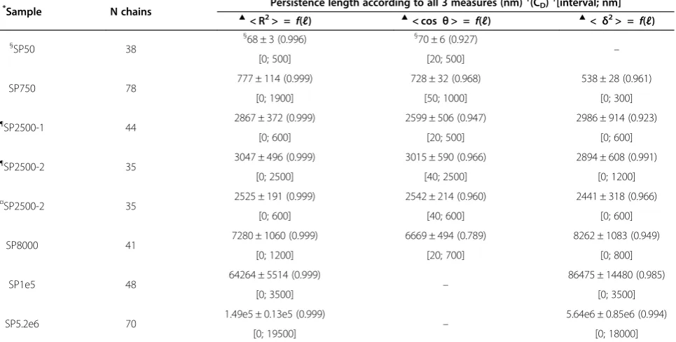
Table 1 Evaluation of the measurement accuracy using synthetic polymers with known persistence lengths as test samples
*
Sample N chains Persistence length according to all 3 measures (nm)
†(CD)‡[interval; nm]
▲< R2
> = f(ℓ) ▲< cos θ> = f(ℓ) ▲< δ2> = f(ℓ)
§
SP50 38
§68 ± 3 (0.996) §70 ± 6 (0.927)
–
[0; 500] [20; 500]
SP750 78 777 ± 114 (0.999) 728 ± 32 (0.968) 538 ± 28 (0.961)
[0; 1900] [50; 1000] [0; 300]
¶
SP2500-1 44 2867 ± 372 (0.999) 2599 ± 506 (0.947) 2986 ± 914 (0.923)
[0; 600] [20; 500] [0; 600]
¶
SP2500-2 35 3047 ± 496 (0.999) 3015 ± 590 (0.966) 2894 ± 608 (0.991)
[0; 2500] [40; 2500] [0; 1200]
¤
SP2500-2 35 2525 ± 191 (0.999) 2542 ± 214 (0.960) 2441 ± 318 (0.966)
[0; 600] [40; 600] [0; 600]
SP8000 41 7280 ± 1060 (0.999) 6669 ± 494 (0.789) 8262 ± 1083 (0.949)
[0; 1200] [20; 700] [0; 800]
SP1e5 48 64264 ± 5514 (0.999) – 86475 ± 14480 (0.985)
[0; 3500] [0; 3500]
SP5.2e6 70 1.49e5 ± 0.13e5 (0.999) – 5.64e6 ± 0.85e6 (0.994)
[0; 19500] [0; 18000]
Refer to Additional file1: Note S4 and Table S1 for details on how the data in this table was generated withSynchainsand analyzed withEasyworm. *
Each number in the sample names corresponds to the persistence length P (in nm) that was used to generate one particular synthetic polymer (SP),e.g.for SP50, P was set to 50 nm.
†C
Dis the coefficient of determination (usually noted“R 2
”but not here because R is already used to refer to the end-to-end distance).
‡[interval] is the range of distanceℓ(along the chain contour) on which each fit was made.
▲Mean square of the end-to-end distance R, tangent-tangent correlations < cosθ> and mean square of the deviationsδto secant midpoint, as described in Eqs.1–3.
§
We excluded chains displaying non-self-avoiding random walk from the analysis of SP50 chains (see Additional file1: Figure S5). Therefore the value of 70 nm for P was expected [3].
¶
SP2500-1 and SP2500-2 differ by their contour length (respectively 0.4 ± 0.2 and 5.3 ± 2.8μm). ¤
Equilibration on the 2D surface
Easyworm2 contains two functions that can help to de-termine whether or not the chains fully equilibrate in 2D (Figure 3). The first one calculates the ratio of the even moments, i.e. the kurtosis of the distribution of the θ angle (Figure 3a). If the chains fully equilibrate in 2D, then theθ distribution is Gaussian [3], and in the range where angles θ are still fully correlated (i.e., ℓ ≤ P and < cosθ> ≥ 0.6, see Figure 4), the kurtosis results in:
<θ4ð Þℓ > 2D
<θ2ð Þℓ >2 2D
¼ 3 ð5Þ
For distances ℓ greater than P, the kurtosis does not equal to 3 anymore and starts decreasing. When theθ an-gles become completely uncorrelated (i.e., < cosθ> = 0), then the distribution ofθ is uniform, that is, all θ angles are equiprobable. Only when this condition is fully met the kurtosis equals 1.8 (see Additional file 1: Figure S4 for more details).
Another function implemented in Easyworm allows for the fast determination of the slope of < R > as a func-tion of ℓ on any given range of ℓ (Figure 3b). Provided the contour length interval defined by the user to calcu-late this slope (corresponding to a scaling or fractal ex-ponent [8]) is located above the persistence length (i.e.
for ℓ > P), the slope is equal to 0.75 for a self-avoiding random walk in 2D [8]. We note that for our software, in practice, this measurement is accurate only for con-tour length values comprised between P and ~3P, since above 3P the number of data points available are usually too low to produce a measurement that is statistically significant.
Results and performance evaluation
We usedin silicopolymers (seeAdditional toolssection) in order to test the accuracy of the measurements made by Easyworm. The benchmarks (see Table 1) indicate that Easyworm is able to provide reliable results over a very wide range of persistence lengths P from that of DNA (P≈50 nm [3]) to that of microtubules (P≈ 5.2 mm [2]). In another test performed on amyloid fi-brils generated in vitro, we determined that relatively good precision on the measurements of P can be ob-tained with a minimum of 50–60 chains that have con-tour length CL~1.0 ± 0.5 nm (Figure 4). The number of
chains required will be higher if CL is lower. As
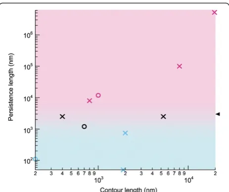
Easy-worm can be used to derive persistence lengths varying over several orders of magnitude, we included a graph-ical guide that provides the user with indications on which measure to use depending on the persistence length of the sample (Figure 5). For instance, when con-sidering fibrils having P > 5 μm, monitoring the end-to-end distance R along the polymer contour is not as
efficient as monitoring the deviations δ from the poly-mer to secant midpoints (see Table 1).
Conclusions
Easyworm is a tool for researchers in need of a fast and ready-to-use program in order to determine the persist-ence length and derive the elastic modulus of their poly-mers, whether these are amyloid fibrils [9] or any nano- or micro-filaments. In addition to determining the mechan-ical properties, Easyworm also provides complementary tools to analyze polymer contour lengths, create synthetic polymers, visualize polymers and generate output files for plotting purposes.
Additional file
Additional file 1:(Easyworm_SuppInfo.pdf) is available with the online version of this article.It contains Additional file Methods, Table S1, Figures S1-S5, Notes S1-S4 (including step-by-step instructions to use the software), and a list of References.
Competing interests
The authors declare no competing interests.
Figure 5Graphical guide indicating which measure should be used to derive the persistence length.The crosses (synthetic chains of known persistence length) and circles (experimental polymers) correspond to data points that are given in Table 1 and Additional file 1: Table S1. Light blue markers represent the samples for which the most reliable calculations of persistence length are achieved by measuring < cosθ> and/or < R2>, whereas purple markers indicate
samples for which measuring <δ2> provides the best estimation of
the persistence length. Black markers indicate samples for which all measures provided reliable results. Therefore, the light blue region indicates where measures of < cosθ> and/or < R2> should be used to
provide the most reliable value for the persistence length, whereas the pink region indicates where measure of <δ2> should be used. Note
Authors’contributions
GL developed the software from TPJK’s initial code. GL and JBK tested the software. HBL and JG advised on the methods. GL wrote the manuscript. All authors commented and edited the manuscript. All authors have read and approved the final manuscript.
Authors’information
GL is a postdoctoral research fellow in the laboratories of JG and HBL at the University of British Columbia (Canada). JBK is a student in TPJK’s laboratory at the University of Cambridge (UK). HBL is an associate professor in Chemistry, TPJK a lecturer in Physical Chemistry, and JG an assistant professor in Biochemistry.
Acknowledgments
This work was financially supported by PrioNet Canada, the Canadian Institutes of Health Research (CIHR), and the Natural Sciences and Engineering Research Council of Canada (NSERC). We thank anonymous reviewers for their helpful comments.
Author details
1Centre for High-Throughput Biology, University of British Colombia,
Vancouver, BC V6T 1Z4, Canada.2Department of Chemistry, University of British Columbia, Vancouver, BC V6T 1Z1, Canada.3Department of
Biochemistry & Molecular Biology, University of British Colombia, Vancouver, BC V6T 2A1, Canada.4Department of Chemistry, University of Cambridge,
Cambridge CB2 1EW, UK.
Received: 23 December 2013 Accepted: 2 July 2014 Published: 10 July 2014
References
1. Doi M, Edwards SF:The Theory of Polymer Dynamics.New York: Oxford University Press Inc.; 1986.
2. Gittes F, Mickey B, Nettleton J, Howard J:Flexural rigidity of microtubules and actin-filaments measured from thermal fluctuations in shape.J Cell Biol1993,120:923–934.
3. Rivetti C, Guthold M, Bustamante C:Scanning force microscopy of DNA deposited onto mica: Equilibration versus kinetic trapping studied by statistical polymer chain analysis.J Mol Biol1996,264:919–932. 4. Grinthal A, Kang SH, Epstein AK, Aizenberg M, Khan M, Aizenberg J:
Steering nanofibers: An integrative approach to bio-inspired fiber fabrication and assembly.Nano Today2012,7:35–52.
5. Knowles TPJ, Buehler MJ:Nanomechanics of functional and pathological amyloid materials.Nat Nanotechnol2011,6:469–479.
6. Easyworm free software.[http://www.chibi.ubc.ca/faculty/joerg-gsponer/ gsponer-lab/software/easyworm]
7. Efron B, Gong G:A leisurely look at the bootstrap, the jackknife, and cross-validation.Am Stat1983,37:36–48.
8. Valle F, Favre M, De Los Rios P, Rosa A, Dietler G:Scaling exponents and probability distributions of DNA end-to-end distance.Phys Rev Lett2005,
95:158105.
9. Lamour G, Yip CK, Li H, Gsponer J:High Intrinsic Mechanical Flexibility of Mouse Prion Nanofibrils Revealed by Measurements of Axial and Radial Young’s Moduli.ACS Nano2014,8:3851–3861.
doi:10.1186/1751-0473-9-16
Cite this article as:Lamouret al.:Easyworm: an open-source software tool to determine the mechanical properties of worm-like chains.Source
Code for Biology and Medicine20149:16. Submit your next manuscript to BioMed Central
and take full advantage of:
• Convenient online submission
• Thorough peer review
• No space constraints or color figure charges
• Immediate publication on acceptance
• Inclusion in PubMed, CAS, Scopus and Google Scholar
• Research which is freely available for redistribution