R E S E A R C H A R T I C L E
Open Access
A simulation study for comparing testing
statistics in response-adaptive randomization
Xuemin Gu
1, J Jack Lee
2*Abstract
Background:Response-adaptive randomizations are able to assign more patients in a comparative clinical trial to the tentatively better treatment. However, due to the adaptation in patient allocation, the samples to be compared are no longer independent. At large sample sizes, many asymptotic properties of test statistics derived for
independent sample comparison are still applicable in adaptive randomization provided that the patient allocation ratio converges to an appropriate target asymptotically. However, the small sample properties of commonly used test statistics in response-adaptive randomization are not fully studied.
Methods:Simulations are systematically conducted to characterize the statistical properties of eight test statistics in six response-adaptive randomization methods at six allocation targets with sample sizes ranging from 20 to 200. Since adaptive randomization is usually not recommended for sample size less than 30, the present paper focuses on the case with a sample of 30 to give general recommendations with regard to test statistics for contingency tables in response-adaptive randomization at small sample sizes.
Results:Among all asymptotic test statistics, the Cook’s correction to chi-square test (TMC) is the best in attaining the nominal size of hypothesis test. The William’s correction to log-likelihood ratio test (TML) gives slightly inflated type I error and higher power as compared withTMC, but it is more robust against the unbalance in patient allocation.TMCandTMLare usually the two test statistics with the highest power in different simulation scenarios. When focusing onTMC andTML, the generalized drop-the-loser urn (GDL) and sequential estimation-adjusted urn (SEU) have the best ability to attain the correct size of hypothesis test respectively. Among all sequential methods that can target different allocation ratios, GDL has the lowest variation and the highest overall power at all allocation ratios. The performance of different adaptive randomization methods and test statistics also depends on allocation targets. At the limiting allocation ratio of drop-the-loser (DL) and randomized play-the-winner (RPW) urn, DL outperforms all other methods including GDL. When comparing the power of test statistics in the same randomization method but at different allocation targets, the powers of likelihood-ratio, relative-risk, log-odds-ratio, Wald-type Z, and chi-square test statistics are maximized at their corresponding optimal allocation ratios for power. Except for the optimal allocation target for log-relative-risk, the other four optimal targets could assign more patients to the worse arm in some simulation scenarios. Another optimal allocation target,RRSIHR, proposed by Rosenberger and Sriram (Journal of Statistical Planning and Inference, 1997) is aimed at minimizing the number of failures at fixed power using Wald-type Z test statistics. Among allocation ratios that always assign more patients to the better treatment,RRSIHR usually has less variation in patient allocation, and the values of variation are consistent across all simulation scenarios. Additionally, the patient allocation atRRSIHR is not too extreme. Therefore,
RRSIHRprovides a good balance between assigning more patients to the better treatment and maintaining the overall power.
Conclusion:The Cook’s correction to chi-square test and Williams’correction to log-likelihood-ratio test are generally recommended for hypothesis test in response-adaptive randomization, especially when sample sizes are small.
* Correspondence: [email protected] 2
Department of Biostatistics, Division of Quantitative Sciences, The University of Texas MD Anderson Cancer Center, PO Box 301402, Unit 1411, Houston, Texas 77230-1402, USA
The generalized drop-the-loser urn design is the recommended method for its good overall properties. Also recommended is the use of theRRSIHRallocation target.
Background
The response-adaptive randomization (RAR) in clinical trials is a class of flexible ways of assigning treatment to new patients sequentially based on available data. The RAR adjusts the allocation probabilities to reflect the interim results of the trial, thereby allowing patients to benefit from the interim knowledge as it accumulates in the trial. In practice, unequal allocation probabilities are generated based on the current assessment of treatment efficacy, which results in more patients being assigned to the treatment that is putatively superior.
Many RAR designs have been proposed over the years [1-13]. The two key issues extensively investigated are the evaluations of parameter estimations and hypothesis testing. Due to the dependency of assigning new patients based on observed data at that time, conven-tional estimates of treatment effect are often biased; therefore, efforts have been made to quantify and cor-rect estimation bias [14,15]. Recent theoretical works have been focused on solving problems encountered in practice, which includes delayed response, implementa-tion for multi-arm trials, and incorporating covariates, etc. [1,3,11,16-18]. Many recent theoretical develop-ments are summarized in [19]. Additionally, in order to compare treatment efficacies through hypothesis testing, studies have been conducted on power comparisons and sample size calculations under the framework of adap-tive randomization [20-24]. However, most of the works are based on large sample sizes, and focus on asymptotic properties [4,12,22,25,26]. But these properties have not been fully studied with small sample sizes. The mathe-matical challenge imposed by correlated data makes it extremely difficult to derive exact solutions for finite samples. Up to now, only limited results on exact solu-tions have been available [15,27], and computer simula-tion has to be relied upon when sample size is small [23,24], which is often the case in early phase II trials.
Each RAR design has its own objective, and there are both advantages and disadvantages associated with that objective. It is not our purpose to give a comprehensive assessment of different designs by comparing their advantages and disadvantages. Instead, the primary objective of the present study is to characterize the small sample properties of RAR based on a frequentist approach. In particular, we focus on comparing the per-formance of commonly used test statistics in RAR of two-arm comparative trials with a binary outcome. Due to the departure from normality caused by data correla-tion and the discrete nature of a binary outcome,
hypothesis tests usually can not be controlled at any given levels of nominal significance. Thus, to make our simulation comparison more relevant, our assessment of hypothesis testing methods and RAR procedures is based on the calculation of both statistical power and the comparison to the nominal type I error rate. Several RAR methods studied in our simulations can assign patients according to a given allocation target, which may be optimal in terms of maximizing the power or minimizing the expected treatment failure. Therefore, we also compare the properties of test statistics at differ-ent optimal allocation targets.
The remaining parts of this paper are organized into 4 sections. In the Methods Section, we introduce the adaptive randomization procedures, the optimal alloca-tion rates, and the test statistics used in the simulaalloca-tion. In the Results Section, we present the simulation results. We provide a discussion and final recommendations regarding the RAR methods and hypothesis tests in the Discussion and Conclusions Sections.
Methods
In the present section, we briefly describe the randomi-zation methods, asymptotic hypothesis test statistics, and optimal patient allocation targets that are relevant to our simulations. More detailed information can be found in the corresponding references.
Response-based Adaptive Randomization (RAR)
of the same type to the urn; a lack of success leads to the addition of b(>0) balls of the other type to the urn (a =b = 1 in our simulation). The limiting allocation rate of patients on treatment 1 is q2/(q1 +q2), where
q1= 1-p1 andq2 = 1-p2are failure rates, and p1andp2 are success rates (or response rates) for treatments 1 and 2. In the DL model, patients are assigned to a treat-ment based on the type of ball that is drawn; however a treatment failure results in the removal of a treatment ball from the urn, and treatment successes are ignored. Due to the finite probabilities of extinction, immigration balls are added to the urn. If an immigration ball is drawn, an additional ball of each type is added. The sampling process is repeated until a treatment ball is drawn. The DL urn design has the same limiting alloca-tion as the RPW urn, but less variability in patient allo-cation. Both SEU and GDL are urn models allowing fraction number of balls, and can target any allocation rate. For SEU method [13], if the limiting allocation of RPW urn is the target in a two-arm trial, then
q∧i( )i ⎡q∧ ( )i +q∧ ( )i
⎣⎢
⎤ ⎦⎥
/ 1 2 balls of type 2 and q∧ ( )i ⎡q∧ ( )i +q∧ ( )i
⎣⎢
⎤ ⎦⎥
2 / 1 2
balls of type 1 are added to the urn following the alloca-tion of theith patient. Obviously, the response status of the ith patient is related to the contents of SEU urn only through the calculation of q∧ i
( )
1 and q i
∧
( )
2 . For
a two-arm GDL urn model [11], when a treatment ball is drawn, a new patient is assigned accordingly, but the ball will not be returned to the urn. Depending on the response of the patient, the conditional average numbers of balls being added back to the urn areb1 and b2 for treatments 1 and 2, respectively. Therefore, the condi-tional average numbers of type 1 and type 2 balls being taken out of the urn can be defined asd1and d2, where
d1 = 1-b1andd2= 1-b2. Immigration balls are also pre-sent in a GDL urn. Whenever an immigration ball is drawn,a1 anda2balls are added for treatments 1 and 2, respectively. Zhang et al [11] have shown that the limit-ing allocation rate of patients on treatment 1 is
n n a d a d a d 1 1 1 1 1 2 2 →
+ . (1)
The GDL urn becomes a DL urn whena1= 1,a2= 1,
b1=p1, andb2=p2. Although GDL is a general method with different ways of implementation, a convenient approach is taken in our simulation. When a treatment ball is drawn, the ball is not returned, and no ball is added regardless of the response of the patient. When an immi-gration ball is drawn,Cr1andCr2balls of type 1 and 2 are added, whereCis a constant, andr1andr2are allocation targets on treatments 1 and 2, which are estimated sequen-tially using the maximum likelihood estimates (MLE) [11].
The SMLE and doubly-adaptive biased coin design (DBCD) methods can also target any allocation ratios, and SMLE can be implemented as a special case of DBCD method. In DBCD method, the probability of the (i+1)th patient being assigned to treatment 1 is calcu-lated by
Pi g i
n i
i i
+ = ⎛
( )
( )
⎝
⎜⎜ ⎞⎠⎟⎟
1 1 , , (2)
where r1 =n1(i)/iand r(i) are the current allocation rate and estimated allocation rate on treatment 1 [2,3]. The properties of the DBCD depend largely on the selection ofg, which can be considered as a measuring function for the deviation from the allocation target. In the present study, we use the following function suggested by Hu and Zhang [3]:
g r r
r r g g , / / / , ,
(
)
=(
)
(
)
+ −(
)
⎡⎣(
−)
(
−)
⎤⎦(
)
=(
)
=1 1 1
0 1
1 00
(3)
where a is a tuning parameter. Whena approaches infinity, the DBCD becomes deterministic and the patients are assigned to the putatively better treatment with probability 1. When a equals to 0, the MLE of
rbecomes the allocation target, and the DBCD method is essentially the same as the SMLE design proposed by Melfi et al [12].
Hypothesis Tests for Two-Arm Comparative Trials
In two-arm comparative trials, the results of a binary outcome variable can be summarized in a 2 × 2 contin-gency table (Table 1). The following hypothesis test is often conducted to compare treatment efficacy:
H p p
H p p
0 1 2
1 1 2
:
: .
=
≠ (4)
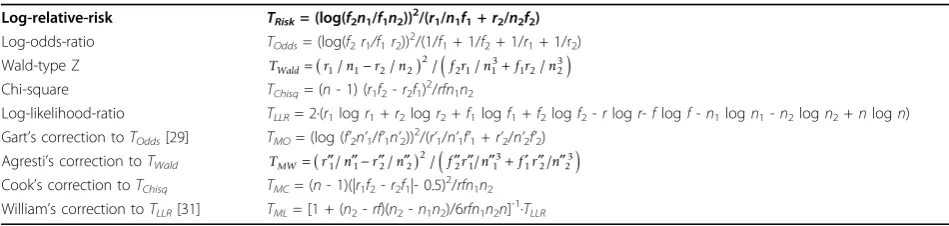
Nine test statistics for the hypothesis test in (4) are given in Table 2. When relative risk (q1/q2) and odds ratio
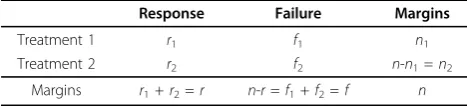
Table 1 Summary of data from a two-arm comparative clinical trial
Response Failure Margins
Treatment 1 r1 f1 n1
Treatment 2 r2 f2 n-n1=n2
Margins r1+r2=r n-r=f1+f2=f n
n: total number of patients;n1,n2: patients on treatment 1 and 2;r: total
number of treatment successes;r1,r2: number of successes on treatment 1
(p1q2/q1p2) are used to quantify the differences between 2 treatment arms, the test statistics are log-relative-risk and log-odds-ratio,TRiskandTOdds, which are asymptotically
distributed as chi-square distribution with one degree of freedom (12). When simple difference is used to measure
the treatment effect, the applicable test statistics are the Wald-type test statisticTWaldand the score-type test
sta-tisticsTChisq, where the variance of simple difference in
response rates is evaluated atH1orH0respectively. Addi-tionally, the test statistics based on the logarithm of likeli-hood ratio (TLLR) can also be constructed. Besides the
5 commonly used test statistics mentioned above, four modified test statistics are also included in Table 2.TMOis
a modified log-odds-ratio test proposed by Gart using the approximation of discrete distributions by their continu-ous analogues [29]. As shown in Table 2,TMOis
essen-tially a modification toTOddsby adding 0.5 to each cell of
a 2 × 2 table. Similarly, Agresti and Caffo proposed a mod-ification toTWaldby adding 1 to each cell of a contingency
table [30], which results in the test statisticTMWin Table
2.TMCis the Cook’s continuity correction to chi-square
test statisticsTChisq. Williams provided a modification to
log-likelihood-ratio testTLLR[31]. The original test
statis-ticTLLR is improved by multiplying a scale factor such
that the null distribution of the new test statisticTMLhas
the same moments as the chi-square distribution.
Since all test statistics in Table 2 are based on 12,
they are asymptotically equivalent and any one of them can be used for large sample sizes. Meanwhile at small sample sizes, an exact test can be conducted if a model is specified for the data given in Table 1. For example, depending on the number of fixed margins predeter-mined for the design, one of the following three models can be applied [32]:
Pr
(
r1| ,n n r1,)
=h r(
1| ,n n r1,)
, (5)Pr
(
r r n n p1, | , 1,)
=h r(
1| ,n n r b r n p1,) (
| ,)
, (6)and
Pr , , | , ,
| , , | , | , ,
r r n n p
h r n n r b r n p b n n p
1 1
1 1 1
(
)
=
(
) (
) (
)
(7)whereh(r1|n, n1,r) represents the hypergeometric dis-tribution ofr1,b(r|n,p) gives the binomial distribution of r under the null hypothesis of equal response rates (H0: p1 =p2 =p), and b(n1|n, r) denotes the binomial distributions of patients on arm 1 with an allocation ratio of r (r1 = 0.5 for equal randomization). The p value of exact test can be calculated by maximizing the probability in (5), (6), or (7) over the two nuisance para-meters, p and r. However, due to data dependency, none of the above three models are directly applicable in adaptive randomization. For example, the allocation ratio rin adaptive randomization is a random variable with unknown distribution, and the binomial distribu-tion ofn1assumed in model (7) is not valid even when the null hypothesis is true. Therefore, in adaptive rando-mization, unconditional exact tests are not available and asymptotic test statistics such as the ones in Table 2 are required for testing the hypothesis in (4).
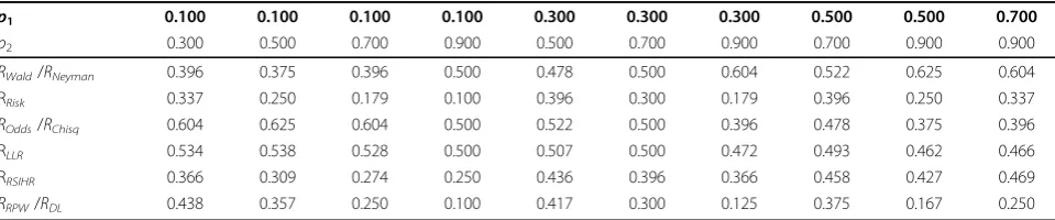
Optimal Allocation Ratios
The SMLE, DBCD, SEU, and GDL methods can be uti-lized to allocate patients based on different allocation targets. The allocation targets simulated in the present study are summarized in Table 3, where RRisk, ROdds,
RWald, RChisq, and RLLR are optimal allocation ratios
maximizing the power ofTRisk, TOdds, TWald,TChisq, and
TLLRrespectively, at fixed sample size. The derivation of
TRisk, TOdds, TWald, TChisq, and TLLR can be found in
[33,34], which is equivalent to minimizing the variance of corresponding test statistic at a fixed total sample size, and consequently the power of that test statistic is maximized.RRSIHRis a recently proposed allocation
tar-get that minimizes the expected total number of failures among all trials with the same power [15,33]. The
Table 2 Test statistics
Log-relative-risk TRisk= (log(f2n1/f1n2))2/(r1/n1f1+r2/n2f2) Log-odds-ratio TOdds= (log(f2r1/f1r2))2/(1/f1+ 1/f2+ 1/r1+ 1/r2)
Wald-type Z TWald=(r1 n1−r2 n2)
(
f r n +f r n)
2
2 1 1 3
1 2 2
3
/ / / / /
Chi-square TChisq= (n- 1) (r1f2-r2f1)2/rfn1n2
Log-likelihood-ratio TLLR= 2·(r1logr1+r2logr2+f1logf1+f2logf2-rlogr-flogf-n1logn1-n2logn2+nlogn) Gart’s correction toTOdds[29] TMO= (log (f’2n’1/f’1n’2))2/(r’1/n’1f’1+r’2/n’2f’2)
Agresti’s correction toTWald TMW= ′′ ′′ − ′′(r1 n1 r2 n′′2)
(
f r′′ ′′ ′′ + ′ ′′ ′′n f r n)
22 1 13 1 2 23
/ / / / /
Cook’s correction toTChisq TMC= (n- 1)(|r1f2-r2f1|- 0.5)2/rfn1n2 William’s correction toTLLR[31] TML= [1 + (n2-rf)(n2-n1n2)/6rfn1n2n]
-1 ·TLLR
r’1=r1+ 0.5,r’2=r2+ 0.5,f’1=f1+ 0.5,f’2=f2+ 0.5,r’=r+ 1,f’+ 1,n’1=n1+ 1,n’2=n2+ 1,n’=n+ 2r”1=r1+ 1,r”2=r2+ 1,f”1=f1+ 1,f”2=f2+ 1,
general theoretical framework and the practical imple-mentation of optimal allocation ink-arm trials with bin-ary outcomes are discussed and demonstrated by Tymofyeyev et al [35], where the optimization can be conducted over different goals. In practice, the perfor-mance of the methodology depends on the chosen RAR procedure. The present simulation study only focuses on two-arm trials, with a goal of maximizing the power or minimizing the total number of failures.
Results
Simulations are conducted at different total numbers of patients ranging from 20 to 200. To simplify the presen-tation, the results for trials with 30 patients are shown here. When patients are less than 30, adaptive randomi-zation is generally not recommended. For sample size of 100 or larger, all methods yield similar properties in general. For all of the urn models, one ball for each treatment is consistently used as the initial contents of the urn. The number of immigration balls is 1 for both the DL and GDL urns. The tuning parameter of DBCD,
a, is fixed at 0 or 2. Whenais 0, it results in the SMLE method. The value of the constantCin GDL is 2, which is equivalent to adding 2 treatment balls on average when an immigration ball is drawn. All simulation results are calculated based on 10,000 replicates.
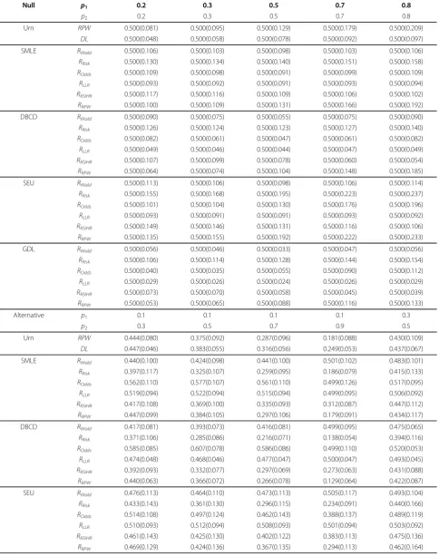
For the purpose of comparison, the true allocation rates are shown in Table 4, and the simulated results for allocation rates on arm 1 are shown in Table 5. Among all RAR methods, DBCD has the best ability to attain
the true allocation target. The comparison between SMLE and DBCD shows that, the allocation becomes more unbalanced and the variation of DBCD decreases with increasing value of tuning exponent a. On the other hand, the patient allocation of SEU results in more balanced mean allocation between two arms with a much larger variation as compared with other RAR methods. The GDL has the lowest variation among the four sequential RAR methods. When RRPW(the same as
RDL) is the allocation target, DL urn method has the
lowest variation in patient allocation, which is consistent with the fact that the lower bound of the estimate of Var(RRPW) is attained by DL urn [4]. The comparison
among allocation targets shows thatRLLRhas the lowest
variation in patient allocation, and the highest variation is usually found atRRPWorRRisk. However, RRPW and
RRisk are usually the top two allocation targets that
assign more patients to the better treatment. RWald,
ROdds, andRLLR assigns more patients to the worse arm
in some simulation cases. Among the three allocation targets that assign more patients to the better treatment (RRSIHR, RRisk and RRPW), RRSIHR has a stable and often
the lowest variation in patient allocation.
The simulation results are obtained for five null cases and ten alternative cases, and Table 6 gives the sum-mary by averaging the results over the five null cases and the ten alternative cases for a given RAR method and at a given allocation target. Detailed simulation results for each test statistic are shown in Tables 7, 8, 9, 10, 11, 12 with one table for each of the six allocation targets. To simplify the presentation, the results are shown only for the four modified test statisticsTMW,
TMO, TMC, TML, and the log-relative-risk test statistic
TRiskbecause they tend to have better performance than
the four corresponding unmodified tests. The qualitative comparisons among test statistics, RAR methods, and allocation targets can be made based on the results in Table 6.
As shown in Table 6 (also see Tables 7, 8, 9, 10, 11, 12), the worst performance can be found in the results ofTMOandTRisk, which are often conservative with less
than nominal type I error rate.TMW is always slightly
conservative across all simulation cases. Overall,TMCis
Table 3 Allocation targets
Optimal allocation ratio (n1/n2) for maximizing powers
RRisk p q1 2/p q2 1
ROdds/RChisq p q2 2/p q1 1 RWald/RNeyman p q1 1/p q2 2
RLLR {q2-p2exp[I1-I2/(p2-p1)]}/{-q1+p1exp[I1-I2/(p2-p1)]}
Other allocation targets
RRPW/RDL q2/q1
RRSIHR p1/p2 (Minimize the number of failure at fixed
power ofTWald)
I1=p1log(p1) +q1log (q1),I2=p2log(p2) +q2log(q2)
Table 4 Asymptotic allocation rates on arm 1 calculated from truep1andp2
p1 0.100 0.100 0.100 0.100 0.300 0.300 0.300 0.500 0.500 0.700
p2 0.300 0.500 0.700 0.900 0.500 0.700 0.900 0.700 0.900 0.900
RWald/RNeyman 0.396 0.375 0.396 0.500 0.478 0.500 0.604 0.522 0.625 0.604
RRisk 0.337 0.250 0.179 0.100 0.396 0.300 0.179 0.396 0.250 0.337
ROdds/RChisq 0.604 0.625 0.604 0.500 0.522 0.500 0.396 0.478 0.375 0.396
RLLR 0.534 0.538 0.528 0.500 0.507 0.500 0.472 0.493 0.462 0.466
RRSIHR 0.366 0.309 0.274 0.250 0.436 0.396 0.366 0.458 0.427 0.469
Table 5 Mean and standard deviation (in parenthesis) of allocation rate on arm 1 forn= 30
Null p1 0.2 0.3 0.5 0.7 0.8
p2 0.2 0.3 0.5 0.7 0.8
Urn RPW 0.500(0.081) 0.500(0.095) 0.500(0.129) 0.500(0.179) 0.500(0.209)
DL 0.500(0.048) 0.500(0.058) 0.500(0.078) 0.500(0.092) 0.500(0.097)
SMLE RWald 0.500(0.106) 0.500(0.103) 0.500(0.098) 0.500(0.103) 0.500(0.106)
RRisk 0.500(0.130) 0.500(0.134) 0.500(0.140) 0.500(0.151) 0.500(0.158)
ROdds 0.500(0.109) 0.500(0.098) 0.500(0.091) 0.500(0.099) 0.500(0.109)
RLLR 0.500(0.093) 0.500(0.092) 0.500(0.091) 0.500(0.093) 0.500(0.094)
RRSIHR 0.500(0.117) 0.500(0.116) 0.500(0.109) 0.500(0.106) 0.500(0.102)
RRPW 0.500(0.100) 0.500(0.109) 0.500(0.131) 0.500(0.166) 0.500(0.192)
DBCD RWald 0.500(0.090) 0.500(0.075) 0.500(0.055) 0.500(0.075) 0.500(0.090)
RRisk 0.500(0.126) 0.500(0.124) 0.500(0.123) 0.500(0.127) 0.500(0.140)
ROdds 0.500(0.082) 0.500(0.061) 0.500(0.047) 0.500(0.061) 0.500(0.082)
RLLR 0.500(0.049) 0.500(0.046) 0.500(0.044) 0.500(0.047) 0.500(0.049)
RRSIHR 0.500(0.107) 0.500(0.099) 0.500(0.078) 0.500(0.060) 0.500(0.054)
RRPW 0.500(0.064) 0.500(0.074) 0.500(0.104) 0.500(0.148) 0.500(0.185)
SEU RWald 0.500(0.113) 0.500(0.106) 0.500(0.098) 0.500(0.106) 0.500(0.114)
RRisk 0.500(0.155) 0.500(0.168) 0.500(0.195) 0.500(0.223) 0.500(0.237)
ROdds 0.500(0.101) 0.500(0.104) 0.500(0.130) 0.500(0.176) 0.500(0.196)
RLLR 0.500(0.093) 0.500(0.091) 0.500(0.091) 0.500(0.093) 0.500(0.092)
RRSIHR 0.500(0.149) 0.500(0.146) 0.500(0.131) 0.500(0.116) 0.500(0.106)
RRPW 0.500(0.135) 0.500(0.155) 0.500(0.192) 0.500(0.222) 0.500(0.233)
GDL RWald 0.500(0.056) 0.500(0.046) 0.500(0.033) 0.500(0.047) 0.500(0.056)
RRisk 0.500(0.106) 0.500(0.114) 0.500(0.128) 0.500(0.144) 0.500(0.154)
ROdds 0.500(0.040) 0.500(0.035) 0.500(0.055) 0.500(0.090) 0.500(0.112)
RLLR 0.500(0.029) 0.500(0.026) 0.500(0.024) 0.500(0.026) 0.500(0.029)
RRSIHR 0.500(0.073) 0.500(0.070) 0.500(0.058) 0.500(0.045) 0.500(0.039)
RRPW 0.500(0.053) 0.500(0.065) 0.500(0.088) 0.500(0.116) 0.500(0.133)
Alternative p1 0.1 0.1 0.1 0.1 0.3
p2 0.3 0.5 0.7 0.9 0.5
Urn RPW 0.444(0.080) 0.375(0.092) 0.287(0.096) 0.181(0.088) 0.430(0.109)
DL 0.447(0.046) 0.383(0.055) 0.316(0.056) 0.249(0.053) 0.437(0.067)
SMLE RWald 0.440(0.100) 0.424(0.098) 0.441(0.100) 0.501(0.102) 0.483(0.101)
RRisk 0.397(0.117) 0.325(0.107) 0.259(0.095) 0.186(0.079) 0.415(0.133)
ROdds 0.562(0.110) 0.577(0.107) 0.561(0.110) 0.499(0.126) 0.517(0.095)
RLLR 0.519(0.094) 0.522(0.094) 0.515(0.094) 0.499(0.095) 0.506(0.092)
RRSIHR 0.417(0.108) 0.369(0.100) 0.335(0.093) 0.312(0.087) 0.447(0.112)
RRPW 0.447(0.099) 0.384(0.105) 0.297(0.106) 0.179(0.091) 0.434(0.117)
DBCD RWald 0.417(0.081) 0.393(0.073) 0.416(0.081) 0.499(0.095) 0.475(0.065)
RRisk 0.371(0.106) 0.285(0.086) 0.216(0.071) 0.138(0.054) 0.394(0.116)
ROdds 0.585(0.085) 0.607(0.078) 0.586(0.086) 0.499(0.110) 0.520(0.053)
RLLR 0.474(0.048) 0.468(0.046) 0.477(0.047) 0.500(0.047) 0.493(0.045)
RRSIHR 0.392(0.093) 0.332(0.077) 0.297(0.069) 0.273(0.063) 0.431(0.088)
RRPW 0.440(0.063) 0.366(0.072) 0.266(0.078) 0.129(0.064) 0.422(0.087)
SEU RWald 0.476(0.113) 0.464(0.110) 0.473(0.113) 0.505(0.117) 0.493(0.104)
RRisk 0.433(0.143) 0.361(0.130) 0.296(0.115) 0.234(0.091) 0.440(0.166)
ROdds 0.514(0.108) 0.497(0.124) 0.462(0.143) 0.388(0.137) 0.489(0.119)
RLLR 0.510(0.093) 0.512(0.094) 0.508(0.093) 0.501(0.094) 0.503(0.092)
RRSIHR 0.461(0.143) 0.425(0.130) 0.402(0.122) 0.383(0.113) 0.475(0.136)
the best in attaining the correct type I error rate.TML, is
slightly inflated as compared with chi-square testTMC.
However, the simulation results not shown here indicate thatTMLis very robust against the unbalance in patient
allocation even when sample size is 20. The comparison between different RAR methods shows that the mean type I error of GDL and SEU can usually match the cor-rect size of tests better than other methods when TMC
and TML are used respectively. The type I error of
DBCD is usually the largest one, except atROdds. The
overall type I error of SEU is comparable with GDL. The power comparison of different test statistics indi-cates thatTRisk is the statistic with the highest power at
RRisk but with a much inflated type I error. Except at
RRisk, TMCor TML is the one with the highest power.
Usually, GDL has the highest power and SEU has the
lowest power among all RAR methods. DBCD and SMLE have similar power, but DBCD is more powerful in most cases. At targetRRPW, DL urn has the best
sta-tistical properties. On the average, the target with the lowest power achieved by test statistics is RRisk. The
highest overall power can usually be achieved by test statistics at RRSIHRandRLLR, butRLLRhas the
disadvan-tage of assigning more patients to the worse treatment in some cases.
Discussion
In response-adaptive randomization, the assignment of a new patient depends on the treatment outcomes of patients previously enrolled in the trial. Delayed responses are often encountered in practice. Recently, the problem of delayed response in multi-arm
Table 5: Mean and standard deviation (in parenthesis) of allocation rate on arm 1 forn= 30(Continued)
GDL RWald 0.450(0.051) 0.437(0.046) 0.452(0.051) 0.500(0.058) 0.486(0.040)
RRisk 0.397(0.093) 0.320(0.085) 0.251(0.071) 0.181(0.055) 0.407(0.114)
ROdds 0.527(0.043) 0.508(0.053) 0.454(0.072) 0.341(0.080) 0.484(0.045)
RLLR 0.517(0.027) 0.521(0.026) 0.515(0.027) 0.500(0.028) 0.505(0.024)
RRSIHR 0.431(0.065) 0.389(0.057) 0.362(0.051) 0.342(0.047) 0.454(0.062)
RRPW 0.454(0.052) 0.399(0.063) 0.329(0.067) 0.236(0.059) 0.444(0.075)
Alternative p1 0.3 0.3 0.5 0.5 0.7
p2 0.7 0.9 0.7 0.9 0.9
Urn RPW 0.341(0.120) 0.227(0.123) 0.411(0.147) 0.288(0.160) 0.375(0.202)
DL 0.363(0.071) 0.290(0.066) 0.424(0.082) 0.343(0.082) 0.416(0.092)
SMLE RWald 0.500(0.104) 0.559(0.100) 0.517(0.100) 0.576(0.099) 0.558(0.101)
RRisk 0.334(0.124) 0.238(0.109) 0.411(0.139) 0.298(0.131) 0.375(0.149)
ROdds 0.500(0.098) 0.438(0.109) 0.485(0.095) 0.423(0.107) 0.438(0.109)
RLLR 0.499(0.091) 0.483(0.093) 0.495(0.092) 0.477(0.094) 0.481(0.094)
RRSIHR 0.408(0.107) 0.378(0.103) 0.459(0.106) 0.429(0.105) 0.468(0.101)
RRPW 0.343(0.122) 0.209(0.110) 0.405(0.141) 0.255(0.136) 0.332(0.174)
DBCD RWald 0.500(0.075) 0.585(0.081) 0.525(0.065) 0.607(0.073) 0.584(0.081)
RRisk 0.300(0.104) 0.187(0.083) 0.391(0.118) 0.250(0.108) 0.337(0.130)
ROdds 0.501(0.061) 0.413(0.086) 0.480(0.054) 0.394(0.079) 0.414(0.084)
RLLR 0.500(0.046) 0.524(0.047) 0.508(0.045) 0.532(0.046) 0.527(0.048)
RRSIHR 0.387(0.080) 0.353(0.075) 0.453(0.069) 0.417(0.066) 0.464(0.055)
RRPW 0.317(0.095) 0.157(0.082) 0.386(0.118) 0.201(0.112) 0.284(0.158)
SEU RWald 0.502(0.106) 0.535(0.108) 0.509(0.102) 0.540(0.102) 0.532(0.108)
RRisk 0.365(0.154) 0.280(0.126) 0.437(0.197) 0.337(0.171) 0.411(0.212)
ROdds 0.453(0.134) 0.384(0.131) 0.469(0.150) 0.399(0.146) 0.438(0.177)
RLLR 0.500(0.091) 0.493(0.094) 0.498(0.093) 0.490(0.094) 0.490(0.092)
RRSIHR 0.449(0.126) 0.429(0.121) 0.479(0.124) 0.460(0.117) 0.481(0.109)
RRPW 0.408(0.162) 0.326(0.141) 0.456(0.197) 0.366(0.173) 0.423(0.208)
GDL RWald 0.499(0.047) 0.548(0.052) 0.514(0.041) 0.562(0.046) 0.548(0.051)
RRisk 0.319(0.104) 0.220(0.078) 0.397(0.128) 0.274(0.104) 0.356(0.138)
ROdds 0.431(0.064) 0.327(0.072) 0.447(0.071) 0.342(0.080) 0.390(0.102)
RLLR 0.500(0.026) 0.485(0.027) 0.495(0.025) 0.479(0.026) 0.483(0.028)
RRSIHR 0.423(0.056) 0.398(0.052) 0.466(0.052) 0.440(0.046) 0.472(0.038)
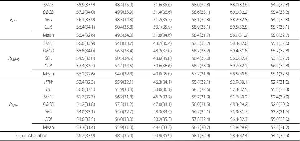
Table 6 The mean and standard deviation (in parenthesis) of type I error and power
Type I error of test statistics
Target Method TMW TRISK TMO TMC TML Row Mean
SMLE 4.4(1.1) 4.6(4.1) 2.0(1.4) 5.0(0.6) 6.8(0.9) 4.6(2.4)
DBCD 4.3(1.4) 5.1(5.1) 1.7(1.7) 4.8(1.2) 7.2(0.8) 4.6(2.9)
RWald SEU 4.0(0.9) 3.4(2.4) 2.3(1.2) 4.8(0.2) 5.6(0.6) 4.0(1.7)
GDL 4.4(0.8) 3.7(3.1) 2.1(1.6) 5.2(0.4) 6.6(1.0) 4.4(2.2)
Mean 4.3(1.0) 4.2(3.6) 2.0(1.4) 5.0(0.7) 6.5(1.0) 4.4(2.3)
SMLE 4.4(1.4) 8.6(3.5) 2.4(1.8) 5.5(1.4) 6.0(1.0) 5.4(2.8)
DBCD 4.6(2.0) 10.2(4.4) 2.6(2.3) 5.7(2.2) 6.5(1.4) 5.9(3.5)
RRisk SEU 3.7(0.8) 7.6(2.3) 2.1(0.8) 5.4(1.3) 5.1(0.4) 4.8(2.2)
GDL 4.2(1.3) 7.9(2.4) 2.4(1.9) 5.4(1.6) 5.8(1.4) 5.1(2.5)
Mean 4.2(1.3) 8.6(3.1) 2.4(1.7) 5.5(1.5) 5.9(1.2) 5.3(2.8)
SMLE 3.7(0.6) 2.4(0.5) 2.9(0.5) 4.8(0.4) 4.5(0.4) 3.7(1.0)
DBCD 3.6(0.7) 2.1(0.8) 3.1(0.7) 4.7(0.3) 4.1(0.2) 3.5(1.1)
ROdds SEU 3.6(0.5) 3.6(0.8) 2.3(0.7) 4.7(0.3) 4.9(0.7) 3.8(1.1)
GDL 3.7(0.8) 3.4(0.8) 3.0(1.1) 5.1(0.4) 4.5(0.4) 3.9(1.0)
Mean 3.7(0.6) 2.9(0.9) 2.8(0.8) 4.9(0.4) 4.5(0.5) 3.7(1.1)
SMLE 4.0(0.6) 2.7(1.2) 2.7(1.0) 5.0(0.2) 5.2(0.6) 3.9(1.3)
DBCD 4.2(0.8) 3.3(2.6) 2.4(1.5) 5.0(0.4) 6.1(0.8) 4.2(1.9)
RLLR SEU 4.0(0.6) 2.8(1.6) 2.4(1.0) 4.9(0.2) 5.4(0.8) 3.9(1.5)
GDL 3.7(0.5) 2.5(1.3) 2.7(1.2) 4.9(0.4) 5.4(0.9) 3.8(1.5)
Mean 3.9(0.6) 2.8(1.6) 2.5(1.1) 5.0(0.3) 5.6(0.8) 4.0(1.5)
SMLE 4.2(1.1) 6.2(4.0) 2.3(1.5) 5.2(0.8) 6.1(0.7) 4.8(2.4)
DBCD 4.3(1.5) 6.9(5.2) 2.0(1.6) 5.2(1.3) 6.5(1.1) 5.0(3.0)
RRSIHR SEU 3.9(0.8) 4.8(3.4) 2.3(1.0) 4.8(0.4) 5.5(0.5) 4.3(1.9)
GDL 4.3(0.9) 4.7(3.0) 2.2(1.6) 5.1(0.6) 6.1(0.9) 4.5(2.0)
Mean 4.2(1.0) 5.7(3.8) 2.2(1.3) 5.1(0.8) 6.1(0.8) 4.6(2.3)
RPW 4.2(0.8) 6.2(0.5) 2.5(1.6) 5.5(1.4) 5.4(0.8) 4.8(1.7)
DL 4.3(0.8) 4.8(1.0) 2.6(1.7) 5.3(0.9) 5.3(0.4) 4.5(1.4)
SMLE 4.2(0.9) 6.5(0.6) 2.8(1.8) 5.4(1.6) 5.1(0.8) 4.8(1.7)
RRPW DBCD 4.3(0.9) 6.7(1.0) 2.9(2.1) 5.7(1.8) 4.8(1.0) 4.9(1.9)
SEU 3.8(0.6) 5.7(1.3) 2.2(0.6) 5.4(0.8) 5.1(0.6) 4.5(1.5)
GDL 4.0(0.8) 5.1(0.6) 2.7(1.6) 5.2(0.7) 5.0(0.8) 4.4(1.3)
Mean 4.1(0.8) 5.8(1.1) 2.6(1.5) 5.4(1.2) 5.1(0.7) 4.6(1.6)
Equal Allocation 4.0(0.5) 2.9(1.7) 2.4(1.0) 5.0(0.2) 5.6(0.8) 4.0(1.5)
Power of test statistics
Target Method TMW TRISK TMO TMC TML Row Mean
SMLE 56.6(34.1) 48.6(35.2) 48.5(36.8) 57.6(33.4) 59.4(31.9) 54.2(33.2)
DBCD 56.9(34.4) 49.5(35.9) 48.0(37.6) 57.7(33.9) 60.2(31.8) 54.5(33.7)
RWald SEU 56.0(34.0) 47.7(34.8) 49.6(36.1) 57.5(33.0) 58.4(32.3) 53.8(32.9)
GDL 57.3(34.0) 50.0(36.2) 50.6(36.9) 58.4(33.2) 60.0(32.0) 55.3(33.3)
Mean 56.7(32.8) 49.0(34.2) 49.2(35.4) 57.8(32.1) 59.5(30.7) 54.4(33.0)
SMLE 53.4(33.2) 57.9(31.5) 45.4(35.2) 56.2(32.7) 55.1(31.1) 53.6(31.7)
DBCD 53.3(33.4) 60.0(30.5) 43.7(36.0) 56.5(32.9) 55.0(31.1) 53.7(31.9)
RRisk SEU 52.5(32.8) 55.3(32.2) 45.9(34.1) 55.2(32.1) 54.2(31.2) 52.6(31.3)
GDL 53.2(33.3) 58.1(31.6) 45.8(35.8) 56.5(32.6) 55.2(31.7) 53.8(31.9)
Mean 53.1(31.9) 57.8(30.3) 45.2(33.9) 56.1(31.3) 54.9(30.1) 53.4(31.5)
SMLE 54.6(33.9) 47.1(34.3) 52.1(34.9) 57.6(32.6) 56.4(32.9) 53.6(32.5)
DBCD 54.8(34.2) 47.3(35.2) 53.4(34.5) 57.8(32.7) 56.5(33.4) 53.9(32.8)
ROdds SEU 54.8(33.5) 50.8(33.8) 50.4(34.8) 57.5(32.5) 56.6(32.2) 54.0(32.1)
GDL 54.6(34.2) 53.0(34.6) 52.5(35.0) 58.1(32.7) 56.8(33.0) 55.0(32.5)
generalized drop-the-loser urn and generalized Fried-man’s urn design is studied for both continuous and dis-continuous outcomes [11,16,17,36]. It is shown that, under reasonable assumption about the delay, the asymptotic properties of adaptive design are not affected by the delay. In the present study, the primary focus is the comparison between commonly used test statistics for 2 × 2 tables. Based on results not shown here, a less extreme allocation with higher variation would be expected when a random delay is assumed. It is assumed that the response status of each of the patients already in the trial is available before the allocation of a new patient in our simulations evaluation.
The RAR methods simulated in the present study are aimed at assigning patients to the better treatment with probabilities higher than what otherwise would be allowed by equal randomization. The price being paid is that the sample sizes on the two comparing arms are no longer fixed, and the adaptation in patient allocation can complicate the statistical inference at the end of the trial. The properties of test statistics will change when the patient allocation ratio changes in adaptive randomi-zation. The power of test statistics shown in the present simulation study is obtained by averaging over trials with an unknown distribution of allocation ratios. As shown in our simulation results, a large deviation from the nominal significance level of the hypothesis test can be found even under the null hypothesis. Therefore, the practice of comparing asymptotic hypothesis testing methods based solely on statistical power under the alternative hypothesis is not recommended. It is
important to compare adaptive randomization methods based on both the type I error rate and the statistical power, especially when the sample size is small.
General recommendations given in the result section are based on the aggregated results across different set-tings. Because the performance of different test statistics, RAR methods, and allocation target are closely related to each other, recommendations under a specific sce-nario can be found based on the detailed simulation results in Tables 7, 8, 9, 10, 11, 12.
Based on simulation results, the Cook’s correction to chi-square test statisticTMC and Williams’correction to
log-likelihood-ratio test TML are recommended to be
used for hypothesis testing at the end of adaptive rando-mization.TMChas good ability to attain the correct
sig-nificance levels, and is relatively robust against the change of RAR method or allocation target. TML has
more robust performance than TMC and has higher
power, but its type I error is slightly inflated as com-pared with TMC. However, TML attains more accurate
type I error than TMC when the sample size is small.
The original Wald-type Z test statistic TWald, which is
very sensitive to patient allocation and has inflated type I error, should be avoided at small sample sizes. On the other hand,TMW, the Argresti’s correction to TWald, and
TMOthe modified log-odds-ratio test are too
conserva-tive and under powered at small sample sizes.
The primary objective of current study is to compare test statistics. Since the recommended test statistics are
TMCand TML, the comparison between RAR methods
and allocation targets are mainly based on these two
Table 6: The mean and standard deviation (in parenthesis) of type I error and power(Continued)
SMLE 55.9(33.9) 48.4(35.0) 51.6(35.6) 58.0(32.8) 58.0(32.6) 54.4(32.8)
DBCD 57.2(34.0) 49.9(35.9) 51.4(36.6) 58.6(33.1) 60.0(32.2) 55.4(33.2)
RLLR SEU 56.1(33.9) 48.5(34.8) 51.2(35.7) 58.1(32.8) 58.2(32.5) 54.4(32.8)
GDL 56.4(34.1) 50.4(35.8) 53.1(35.9) 58.9(33.1) 59.5(32.5) 55.7(33.1)
Mean 56.4(32.6) 49.3(34.0) 51.8(34.6) 58.4(31.7) 58.9(31.2) 55.0(32.7)
SMLE 56.0(33.9) 54.8(33.7) 48.7(36.4) 57.5(33.2) 58.4(32.0) 55.1(32.6)
DBCD 56.8(34.0) 56.3(33.4) 48.2(37.0) 58.2(33.2) 59.4(31.8) 55.7(32.8)
RRSIHR SEU 54.5(33.8) 50.5(34.5) 48.6(35.8) 56.4(33.0) 56.6(32.4) 53.3(32.7)
GDL 57.4(33.7) 54.4(34.5) 50.6(36.6) 58.7(33.0) 59.7(32.1) 56.2(32.8)
Mean 56.2(32.6) 54.0(32.8) 49.0(35.0) 57.7(31.8) 58.5(30.8) 55.1(32.5)
RPW 52.4(32.3) 55.9(32.1) 46.3(34.1) 55.8(32.1) 52.9(30.1) 52.7(31.0)
DL 56.0(33.5) 55.9(33.4) 50.0(36.1) 58.2(32.6) 57.4(32.5) 55.5(32.4)
SMLE 51.7(32.3) 56.2(31.8) 46.7(33.7) 55.7(31.9) 51.7(30.2) 52.4(30.9)
RRPW DBCD 51.2(31.8) 57.3(31.2) 47.0(34.1) 56.0(31.5) 48.3(29.2) 52.0(30.6)
SEU 54.0(33.1) 54.0(32.7) 48.3(34.4) 56.7(32.1) 55.9(31.7) 53.8(31.6)
GDL 54.6(33.5) 56.0(33.0) 50.2(35.3) 57.8(32.4) 56.4(32.3) 55.0(32.0)
Mean 53.3(31.4) 55.9(31.0) 48.1(33.2) 56.7(30.7) 53.8(29.8) 53.5(31.2)
Equal Allocation 56.2(33.9) 48.5(35.0) 50.9(35.9) 58.1(32.9) 58.4(32.4) 54.4(32.9)
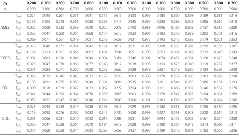
Table 7 Power and type I error atRWald(alpha = 0.05,n= 30)
p1 0.200 0.300 0.500 0.700 0.800 0.100 0.100 0.100 0.100 0.300 0.300 0.300 0.500 0.500 0.700
p2 0.200 0.300 0.500 0.700 0.800 0.300 0.500 0.700 0.900 0.500 0.700 0.900 0.700 0.900 0.900
TMW 0.031 0.048 0.056 0.050 0.033 0.196 0.674 0.953 0.999 0.201 0.600 0.950 0.203 0.680 0.202
TRisk 0.102 0.072 0.039 0.014 0.003 0.326 0.693 0.940 0.996 0.181 0.501 0.798 0.113 0.288 0.024
SMLE TMO 0.007 0.022 0.041 0.024 0.007 0.063 0.492 0.928 0.999 0.162 0.563 0.923 0.161 0.495 0.069
TMC 0.044 0.052 0.056 0.055 0.044 0.231 0.689 0.954 0.999 0.203 0.601 0.952 0.205 0.693 0.235
TML 0.074 0.066 0.055 0.067 0.079 0.308 0.709 0.954 0.999 0.203 0.595 0.951 0.205 0.711 0.309
TMW 0.029 0.050 0.057 0.052 0.026 0.186 0.685 0.957 0.999 0.212 0.607 0.958 0.206 0.696 0.191
TRisk 0.120 0.085 0.041 0.008 0.001 0.361 0.721 0.954 0.998 0.204 0.524 0.811 0.109 0.257 0.010
DBCD TMO 0.004 0.017 0.045 0.017 0.003 0.041 0.462 0.933 0.999 0.169 0.587 0.934 0.164 0.475 0.042
TMC 0.037 0.056 0.058 0.056 0.034 0.211 0.696 0.958 0.999 0.215 0.607 0.959 0.208 0.706 0.215
TML 0.077 0.074 0.059 0.073 0.077 0.311 0.718 0.958 0.999 0.217 0.607 0.959 0.210 0.727 0.315
TMW 0.031 0.045 0.048 0.044 0.030 0.200 0.655 0.946 0.999 0.190 0.583 0.948 0.191 0.675 0.213
TRisk 0.067 0.048 0.033 0.016 0.006 0.259 0.646 0.922 0.991 0.154 0.486 0.812 0.114 0.342 0.046
SEU TMO 0.013 0.026 0.039 0.027 0.011 0.094 0.522 0.921 0.999 0.158 0.553 0.926 0.157 0.533 0.095
TMC 0.046 0.051 0.049 0.050 0.046 0.248 0.675 0.949 0.999 0.195 0.585 0.950 0.195 0.698 0.258
TML 0.062 0.055 0.047 0.055 0.062 0.285 0.683 0.947 0.999 0.190 0.577 0.949 0.193 0.710 0.305
TMW 0.036 0.051 0.051 0.049 0.034 0.223 0.696 0.954 1.000 0.195 0.601 0.958 0.200 0.692 0.214
TRisk 0.075 0.060 0.040 0.010 0.001 0.309 0.703 0.949 0.999 0.184 0.543 0.868 0.124 0.304 0.015
GDL TMO 0.007 0.022 0.046 0.023 0.006 0.077 0.549 0.937 0.999 0.167 0.588 0.945 0.169 0.547 0.077
TMC 0.048 0.057 0.051 0.055 0.047 0.260 0.708 0.955 1.000 0.198 0.602 0.960 0.204 0.705 0.253
TML 0.074 0.064 0.052 0.063 0.076 0.319 0.721 0.956 1.000 0.200 0.602 0.960 0.205 0.720 0.314
For each RAR methods, the results of the following 5 test statistics are shown: Agresti’s correction to Wald-type Z testTMW, log-relative-risk testTRisk, Gart’s
correction to log-odds-ratio testTMO, Cook’s correction to chi-square testTMC, and Williams’correction log-likelihood-ratio testTML.
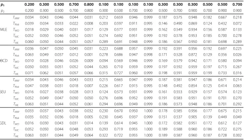
Table 8 Power and type I error atRRisk(alpha = 0.05,n= 30)
p1 0.200 0.300 0.500 0.700 0.800 0.100 0.100 0.100 0.100 0.300 0.300 0.300 0.500 0.500 0.700
p2 0.200 0.300 0.500 0.700 0.800 0.300 0.500 0.700 0.900 0.500 0.700 0.900 0.700 0.900 0.900
TMW 0.024 0.045 0.061 0.051 0.041 0.156 0.615 0.923 0.990 0.185 0.560 0.898 0.189 0.611 0.214
TRisk 0.136 0.105 0.078 0.061 0.050 0.363 0.716 0.945 0.997 0.230 0.588 0.923 0.206 0.612 0.210
SMLE TMO 0.002 0.008 0.032 0.039 0.040 0.022 0.278 0.792 0.988 0.096 0.466 0.903 0.157 0.615 0.220
TMC 0.033 0.047 0.060 0.064 0.068 0.177 0.615 0.923 0.996 0.183 0.570 0.939 0.202 0.701 0.316
TML 0.069 0.071 0.061 0.049 0.051 0.278 0.659 0.921 0.975 0.195 0.543 0.883 0.179 0.621 0.253
TMW 0.018 0.046 0.072 0.054 0.042 0.134 0.617 0.931 0.993 0.198 0.565 0.896 0.199 0.586 0.207
TRisk 0.166 0.123 0.091 0.066 0.062 0.402 0.744 0.951 0.998 0.253 0.606 0.926 0.225 0.649 0.243
DBCD TMO 0.001 0.003 0.030 0.046 0.049 0.004 0.164 0.746 0.994 0.074 0.457 0.904 0.158 0.623 0.248
TMC 0.023 0.047 0.070 0.068 0.077 0.148 0.612 0.928 0.998 0.193 0.575 0.940 0.218 0.707 0.327
TML 0.071 0.083 0.071 0.050 0.050 0.278 0.665 0.928 0.979 0.207 0.549 0.880 0.184 0.596 0.240
TMW 0.026 0.039 0.045 0.043 0.032 0.172 0.598 0.903 0.988 0.178 0.537 0.888 0.183 0.606 0.198
TRisk 0.105 0.092 0.075 0.059 0.049 0.307 0.686 0.935 0.996 0.201 0.546 0.903 0.186 0.581 0.193
SEU TMO 0.009 0.018 0.029 0.027 0.023 0.062 0.372 0.794 0.986 0.121 0.468 0.887 0.146 0.582 0.176
TMC 0.041 0.044 0.050 0.064 0.070 0.209 0.605 0.903 0.994 0.178 0.542 0.922 0.194 0.681 0.289
TML 0.057 0.052 0.047 0.049 0.048 0.266 0.640 0.900 0.981 0.183 0.526 0.879 0.178 0.624 0.245
TMW 0.023 0.043 0.059 0.047 0.038 0.168 0.617 0.929 0.993 0.182 0.558 0.902 0.196 0.580 0.195
TRisk 0.113 0.092 0.076 0.062 0.053 0.347 0.720 0.950 0.998 0.227 0.593 0.928 0.220 0.617 0.213
GDL TMO 0.001 0.006 0.031 0.040 0.042 0.016 0.283 0.831 0.994 0.094 0.473 0.908 0.161 0.604 0.220
TMC 0.030 0.047 0.058 0.064 0.070 0.194 0.618 0.928 0.998 0.180 0.567 0.943 0.214 0.696 0.311
Table 9 Power and type I error atROdds(alpha = 0.05,n= 30)
p1 0.200 0.300 0.500 0.700 0.800 0.100 0.100 0.100 0.100 0.300 0.300 0.300 0.500 0.500 0.700
p2 0.200 0.300 0.500 0.700 0.800 0.300 0.500 0.700 0.900 0.500 0.700 0.900 0.700 0.900 0.900
TMW 0.030 0.040 0.042 0.040 0.031 0.202 0.630 0.935 0.998 0.178 0.562 0.939 0.174 0.637 0.205
TRisk 0.022 0.023 0.030 0.026 0.017 0.143 0.502 0.857 0.984 0.128 0.475 0.884 0.129 0.497 0.112
SMLE TMO 0.024 0.031 0.036 0.031 0.023 0.163 0.587 0.926 0.999 0.154 0.536 0.929 0.151 0.598 0.167
TMC 0.053 0.048 0.043 0.047 0.052 0.283 0.682 0.946 0.999 0.184 0.566 0.947 0.180 0.690 0.285
TML 0.048 0.045 0.040 0.044 0.049 0.266 0.662 0.938 0.998 0.174 0.551 0.941 0.171 0.672 0.270
TMW 0.029 0.040 0.044 0.040 0.028 0.191 0.632 0.940 0.999 0.180 0.572 0.941 0.178 0.644 0.198
TRisk 0.011 0.018 0.032 0.026 0.018 0.085 0.448 0.864 0.994 0.120 0.490 0.906 0.141 0.547 0.134
DBCD TMO 0.026 0.033 0.042 0.031 0.024 0.178 0.609 0.934 0.999 0.165 0.555 0.933 0.161 0.619 0.185
TMC 0.052 0.046 0.045 0.046 0.048 0.280 0.688 0.948 0.999 0.185 0.573 0.949 0.181 0.696 0.284
TML 0.040 0.043 0.043 0.043 0.038 0.244 0.667 0.945 0.999 0.178 0.565 0.944 0.174 0.680 0.252
TMW 0.032 0.041 0.043 0.037 0.030 0.207 0.647 0.935 0.996 0.183 0.562 0.924 0.186 0.636 0.204
TRisk 0.047 0.040 0.035 0.032 0.028 0.214 0.605 0.903 0.993 0.152 0.503 0.894 0.140 0.528 0.146
SEU TMO 0.014 0.026 0.032 0.023 0.020 0.127 0.540 0.900 0.995 0.148 0.520 0.914 0.150 0.587 0.159
TMC 0.049 0.047 0.043 0.047 0.052 0.268 0.676 0.938 0.998 0.187 0.564 0.945 0.191 0.695 0.284
TML 0.059 0.049 0.042 0.044 0.049 0.285 0.677 0.935 0.995 0.182 0.551 0.922 0.183 0.665 0.268
TMW 0.029 0.037 0.049 0.041 0.030 0.203 0.657 0.943 0.999 0.167 0.573 0.929 0.178 0.617 0.192
TRisk 0.024 0.032 0.046 0.035 0.031 0.183 0.625 0.936 0.999 0.158 0.560 0.922 0.165 0.583 0.166
GDL TMO 0.013 0.026 0.043 0.034 0.033 0.124 0.587 0.930 0.999 0.150 0.552 0.928 0.161 0.619 0.204
TMC 0.051 0.047 0.050 0.050 0.058 0.281 0.700 0.948 0.999 0.177 0.579 0.949 0.187 0.695 0.298
TML 0.050 0.047 0.046 0.039 0.043 0.282 0.700 0.947 0.999 0.176 0.563 0.933 0.169 0.652 0.258
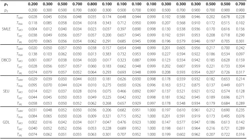
Table 10 Power and type I error atRLLR(alpha = 0.05,n= 30)
p1 0.200 0.300 0.500 0.700 0.800 0.100 0.100 0.100 0.100 0.300 0.300 0.300 0.500 0.500 0.700
p2 0.200 0.300 0.500 0.700 0.800 0.300 0.500 0.700 0.900 0.500 0.700 0.900 0.700 0.900 0.900
TMW 0.034 0.043 0.046 0.044 0.031 0.212 0.659 0.946 0.999 0.187 0.575 0.948 0.182 0.667 0.218
TRisk 0.039 0.034 0.033 0.022 0.008 0.203 0.597 0.911 0.995 0.146 0.490 0.869 0.124 0.432 0.072
SMLE TMO 0.018 0.029 0.040 0.031 0.017 0.129 0.577 0.931 0.999 0.162 0.549 0.934 0.156 0.587 0.133
TMC 0.052 0.050 0.046 0.052 0.051 0.274 0.692 0.951 0.999 0.192 0.578 0.953 0.185 0.700 0.278
TML 0.060 0.050 0.044 0.051 0.057 0.289 0.691 0.948 0.999 0.186 0.567 0.950 0.181 0.698 0.289
TMW 0.036 0.047 0.050 0.045 0.031 0.223 0.688 0.957 0.999 0.192 0.591 0.956 0.192 0.697 0.225
TRisk 0.063 0.049 0.037 0.012 0.001 0.278 0.686 0.947 0.998 0.171 0.528 0.872 0.129 0.356 0.026
DBCD TMO 0.010 0.028 0.046 0.026 0.009 0.094 0.569 0.946 0.999 0.169 0.579 0.942 0.171 0.580 0.094
TMC 0.050 0.055 0.051 0.052 0.044 0.265 0.710 0.959 0.999 0.197 0.592 0.959 0.197 0.715 0.267
TML 0.071 0.062 0.051 0.057 0.066 0.315 0.727 0.960 0.999 0.198 0.591 0.959 0.199 0.733 0.316
TMW 0.034 0.043 0.046 0.043 0.033 0.215 0.665 0.947 0.999 0.187 0.581 0.947 0.186 0.671 0.214
TRisk 0.047 0.038 0.031 0.018 0.007 0.226 0.617 0.915 0.995 0.148 0.492 0.854 0.125 0.414 0.063
SEU TMO 0.016 0.027 0.038 0.028 0.013 0.124 0.573 0.931 0.999 0.161 0.553 0.929 0.157 0.574 0.123
TMC 0.052 0.049 0.047 0.050 0.050 0.276 0.696 0.952 0.999 0.191 0.583 0.951 0.191 0.701 0.270
TML 0.063 0.051 0.044 0.052 0.061 0.294 0.696 0.949 0.999 0.186 0.573 0.948 0.186 0.701 0.292
TMW 0.033 0.037 0.043 0.038 0.032 0.230 0.670 0.950 1.000 0.178 0.585 0.956 0.177 0.675 0.215
TRisk 0.035 0.032 0.036 0.018 0.005 0.230 0.645 0.937 0.999 0.151 0.537 0.905 0.139 0.449 0.049
GDL TMO 0.016 0.030 0.043 0.031 0.014 0.139 0.614 0.945 1.000 0.172 0.582 0.951 0.172 0.612 0.127
TMC 0.052 0.050 0.044 0.048 0.053 0.293 0.719 0.955 1.000 0.189 0.588 0.960 0.186 0.722 0.275
selected test statistics. Among SMLE, DBCD, SEU, and GDL methods, GDL seems to be the best one due to its ability to attain the correct size of hypothesis test and comparatively higher overall power at most allocation targets. Therefore, GDL is the recommended RAR method. The sequential estimation-adjusted urn (SEU) method is comparable with GDL in controlling the type I error. However, SEU is often under powered, and the high variation in patient allocation makes it less useful in practice. The DBCD method with tuning exponent a equal to 2 is the best in targeting the true allocation ratio. WhenTMCis the test statistic, DBCD has slightly
inflated type I error and slightly lower power as com-pared with GDL. Therefore, among values ofa, the bal-ances among controlling the type I error, obtaining higher power, and targeting a given allocation ratio can be reached whena is equal to 2. The simulation com-parison of statistical power for different RAR methods also indicates that DL urn has the best statistical proper-ties atRRPW, mainly due to its low variation in patient
allocation.
The statistical characteristics of hypothesis tests and RAR methods also depend on allocation targets. At
RWald, ROdds, andRLLR targets, more patients could be
assigned to the inferior treatment in certain parameter spaces. In contrast,RRisk,RRPW, andRRSIHR always assign
more patients to the better treatment. However, due to the more extreme allocation of RRisk and RRPW, both
power and type I error ofRRisk and RRPW will suffer as
compared withRRSIHR. On the other hand, the variation
of patient allocation atRRISHR is relatively small with a
stable value across all simulation scenarios. Additional, among all designs with similar power using Wald-type test statistic,RRSIHR allocation ration can achieve fewer
failures in the whole trial. Therefore,RRSIHR is
recom-mended among all the allocation targets in the present study.
In addition to the frequentist development on the response adaptive randomization, Bayesian decision the-oretic methods has also been proposed in the context of bandit problem. The concept of “patient horizon” was brought up to include future patients to whom the cur-rent study results might be applied. The goal is to maxi-mize the total number of success in patients enrolled in the study with or without including the patient horizon. More detailed exposition of Bayesian methods for response adaptive randomization is beyond the scope of this paper and interested readers should consult the original work on this topic [37-40].
Conclusion
The Cook’s correction to chi-square test and Williams’ correction to log-likelihood-ratio test are recommended for hypothesis test of RAR at small sample sizes. Among all the RAR methods compared, GDL method has better statistical properties in controlling type one error and
Table 11 Power and type I error atRRSIHR(alpha = 0.05,n= 30)
p1 0.200 0.300 0.500 0.700 0.800 0.100 0.100 0.100 0.100 0.300 0.300 0.300 0.500 0.500 0.700
p2 0.200 0.300 0.500 0.700 0.800 0.300 0.500 0.700 0.900 0.500 0.700 0.900 0.700 0.900 0.900
TMW 0.028 0.045 0.056 0.048 0.035 0.174 0.648 0.944 0.999 0.192 0.588 0.946 0.202 0.678 0.228
TRisk 0.118 0.085 0.058 0.034 0.018 0.343 0.712 0.950 0.999 0.207 0.568 0.910 0.172 0.515 0.102
SMLE TMO 0.004 0.012 0.040 0.034 0.023 0.037 0.397 0.890 0.998 0.130 0.538 0.936 0.170 0.616 0.156
TMC 0.038 0.049 0.056 0.057 0.057 0.200 0.657 0.945 0.999 0.192 0.591 0.953 0.208 0.718 0.290
TML 0.070 0.065 0.056 0.054 0.062 0.291 0.685 0.945 0.998 0.196 0.579 0.946 0.197 0.705 0.301
TMW 0.020 0.050 0.057 0.050 0.038 0.157 0.654 0.948 0.999 0.201 0.605 0.956 0.217 0.700 0.242
TRisk 0.138 0.103 0.062 0.030 0.013 0.383 0.732 0.953 0.999 0.227 0.594 0.922 0.186 0.534 0.097
DBCD TMO 0.001 0.007 0.038 0.034 0.020 0.017 0.323 0.887 0.999 0.123 0.554 0.942 0.185 0.628 0.159
TMC 0.028 0.056 0.057 0.057 0.060 0.183 0.662 0.948 0.999 0.202 0.607 0.959 0.221 0.733 0.304
TML 0.074 0.079 0.057 0.052 0.064 0.293 0.693 0.948 0.999 0.208 0.593 0.954 0.207 0.726 0.317
TMW 0.029 0.039 0.050 0.044 0.033 0.181 0.626 0.930 0.998 0.178 0.559 0.932 0.182 0.653 0.214
TRisk 0.095 0.070 0.044 0.024 0.010 0.275 0.650 0.926 0.996 0.163 0.512 0.875 0.137 0.449 0.071
SEU TMO 0.014 0.021 0.037 0.028 0.016 0.075 0.466 0.892 0.997 0.137 0.521 0.921 0.152 0.574 0.128
TMC 0.044 0.045 0.050 0.053 0.049 0.225 0.642 0.932 0.998 0.181 0.562 0.945 0.189 0.696 0.271
TML 0.058 0.053 0.050 0.052 0.062 0.268 0.657 0.929 0.997 0.178 0.548 0.934 0.179 0.684 0.289
TMW 0.031 0.048 0.052 0.050 0.036 0.206 0.682 0.951 1.000 0.197 0.610 0.961 0.212 0.690 0.235
TRisk 0.084 0.065 0.050 0.026 0.009 0.321 0.715 0.952 1.000 0.201 0.591 0.919 0.173 0.495 0.076
GDL TMO 0.002 0.016 0.042 0.034 0.017 0.047 0.476 0.923 1.000 0.147 0.577 0.947 0.186 0.613 0.142
TMC 0.040 0.052 0.052 0.056 0.053 0.228 0.689 0.952 1.000 0.198 0.611 0.964 0.216 0.721 0.289
maintaining high statistical power. The RSIHR allocation target provides a good balance between assigning more patients to the better treatment and maintaining a high overall power.
Abbreviations
RAR: Response-adaptive randomization; RPW: Randomized play-the-winner; DL: Drop-the-loser; DBCD: Doubly-adaptive biased coin design; SMLE: Sequential maximum likelihood estimation design; SEU: Sequential estimation-adjusted urn; GDL: Generalized drop-the-loser urn; RSIHR: Optimal allocation target minimizing total numbers of failure for Wald-type test statistics at fixed power; MLE: Maximum likelihood estimate.
Acknowledgements
This work was supported in part by grants CA16672 from the National Cancer Institute and W81XWH-06-1-0303 and W81XWH-07-1-0306 from the Department of Defense. The authors thank Dr. Lunagomez for helpful discussions. The authors also thank Ms. Lee Ann Chastain for her help, which greatly improved the presentation of our study.
Author details
1Department of Biostatistics, Division of Quantitative Sciences, The University
of Texas MD Anderson Cancer Center, PO Box 301402, Unit 1409, Houston, Texas 77230-1402, USA.2Department of Biostatistics, Division of Quantitative Sciences, The University of Texas MD Anderson Cancer Center, PO Box 301402, Unit 1411, Houston, Texas 77230-1402, USA.
Authors’contributions
XMG conducted the simulation part of the study. Both XMG and JJL participated in designing the study and writing the manuscript. All authors read and approved the final manuscript.
Competing interests
The authors declare that they have no competing interests.
Received: 4 November 2008 Accepted: 5 June 2010 Published: 5 June 2010
References
1. Andersen J, Faries D, Tamura R:A randomized play-the-winner design for multi-arm clinical trials.Communications in Statistics-Theory and Methods 1994,23:309-323.
Table 12 Power and type I error atRRPW(alpha = 0.05,n= 30)
p1 0.200 0.300 0.500 0.700 0.800 0.100 0.100 0.100 0.100 0.300 0.300 0.300 0.500 0.500 0.700
p2 0.200 0.300 0.500 0.700 0.800 0.300 0.500 0.700 0.900 0.500 0.700 0.900 0.700 0.900 0.900
TMW 0.031 0.039 0.050 0.050 0.042 0.191 0.631 0.918 0.966 0.166 0.538 0.859 0.183 0.585 0.204
TRisk 0.071 0.058 0.059 0.061 0.060 0.287 0.683 0.939 0.993 0.193 0.565 0.905 0.197 0.607 0.216
RPW TMO 0.004 0.012 0.032 0.038 0.039 0.047 0.410 0.840 0.967 0.105 0.467 0.867 0.151 0.584 0.196
TMC 0.045 0.042 0.050 0.063 0.075 0.227 0.640 0.921 0.988 0.167 0.546 0.914 0.196 0.680 0.301
TML 0.067 0.050 0.049 0.049 0.053 0.288 0.661 0.916 0.931 0.172 0.523 0.820 0.173 0.573 0.235
TMW 0.032 0.043 0.052 0.050 0.040 0.208 0.658 0.944 0.998 0.183 0.586 0.939 0.204 0.658 0.219
TRisk 0.057 0.051 0.055 0.048 0.032 0.273 0.679 0.947 0.998 0.192 0.588 0.935 0.199 0.612 0.164
DL TMO 0.003 0.013 0.038 0.041 0.033 0.047 0.464 0.906 0.998 0.123 0.527 0.934 0.172 0.641 0.193
TMC 0.043 0.045 0.052 0.062 0.064 0.237 0.662 0.944 0.999 0.184 0.592 0.956 0.216 0.723 0.307
TML 0.058 0.050 0.050 0.049 0.056 0.275 0.672 0.943 0.998 0.183 0.567 0.940 0.188 0.688 0.283
TMW 0.027 0.040 0.048 0.049 0.044 0.188 0.626 0.921 0.968 0.167 0.537 0.848 0.175 0.550 0.195
TRisk 0.073 0.062 0.058 0.063 0.072 0.283 0.678 0.936 0.993 0.193 0.563 0.910 0.196 0.617 0.247
SMLE TMO 0.006 0.012 0.031 0.040 0.049 0.054 0.409 0.840 0.969 0.108 0.463 0.864 0.148 0.584 0.229
TMC 0.039 0.044 0.049 0.061 0.079 0.226 0.636 0.922 0.989 0.168 0.547 0.911 0.190 0.671 0.315
TML 0.064 0.054 0.046 0.046 0.047 0.287 0.659 0.917 0.925 0.171 0.519 0.794 0.165 0.528 0.200
TMW 0.031 0.037 0.053 0.049 0.044 0.202 0.635 0.929 0.969 0.181 0.529 0.813 0.173 0.503 0.192
TRisk 0.063 0.054 0.065 0.072 0.081 0.290 0.685 0.942 0.994 0.202 0.572 0.911 0.209 0.640 0.285
DBCD TMO 0.003 0.010 0.033 0.043 0.054 0.041 0.407 0.866 0.981 0.110 0.460 0.856 0.146 0.573 0.257
TMC 0.041 0.040 0.054 0.067 0.083 0.236 0.640 0.930 0.990 0.181 0.543 0.905 0.195 0.660 0.325
TML 0.061 0.048 0.052 0.042 0.036 0.289 0.661 0.925 0.857 0.183 0.511 0.696 0.160 0.407 0.144
TMW 0.033 0.040 0.047 0.041 0.032 0.204 0.633 0.924 0.994 0.183 0.553 0.908 0.185 0.618 0.199
TRisk 0.076 0.059 0.058 0.048 0.043 0.278 0.664 0.929 0.996 0.183 0.529 0.899 0.170 0.564 0.182
SEU TMO 0.012 0.021 0.028 0.027 0.024 0.100 0.467 0.855 0.993 0.130 0.493 0.900 0.143 0.578 0.169
TMC 0.051 0.047 0.050 0.059 0.065 0.251 0.652 0.925 0.997 0.186 0.556 0.933 0.197 0.686 0.286
TML 0.062 0.051 0.048 0.047 0.049 0.293 0.671 0.923 0.992 0.185 0.541 0.904 0.183 0.642 0.251
TMW 0.032 0.045 0.049 0.045 0.032 0.216 0.658 0.937 0.998 0.171 0.576 0.916 0.192 0.602 0.196
TRisk 0.056 0.053 0.053 0.050 0.042 0.281 0.681 0.942 0.998 0.180 0.586 0.927 0.196 0.615 0.197
GDL TMO 0.004 0.017 0.036 0.040 0.037 0.066 0.480 0.900 0.998 0.122 0.525 0.918 0.165 0.622 0.219
TMC 0.044 0.049 0.050 0.058 0.061 0.250 0.666 0.939 0.999 0.173 0.584 0.948 0.206 0.700 0.314
2. Eisele JR:The doubly adaptive biased coin design for sequential clinical trials.Journal of Statistical Planning and Inference1994,38:249-262. 3. Hu FF, Zhang LX:Asymptotic properties of doubly adaptive biased coin
designs for multi-treatment clinical trials.Annals of Statistics2004, 32(1):268-301.
4. Ivanova S, Rosenberger WF, Durham S, Flournoy N:A birth and death urn for randomized clinical trials: asymptotic methods.Sankhya: The Indian Journals of Statistics2000,62(B):104-118.
5. Li W, Durham SD, Flournoy N:Randomized Pôlya urn.1996 Proceedings of the Biopharmaceutical Section of the American Statistical Association: 1997; Alexandria: American Statistical Association1997, 166-170.
6. Rosenberger WF, Stallard N, Ivanova A, Harper CN, Ricks ML:Optimal adaptive designs for binary response trials.Biometrics2001,57:909-913. 7. Wei LJ:The generalized Polya’s urn design for sequential medical trials.
Annals of Statistics1979,7:291-296.
8. Wei LJ, Durham SD:The randomized play-the-winner rule in medical trials.Journal of American Statistical Association1978,85:156-162. 9. Yang Y, Zhu D:Randomized allocation with nonparametric estimation for
a multi-armed bandit problem with covariates.Annals of Statistics2002, 30:100-121.
10. Zelen M:Play the winner rule and the controlled clinical trial.Journal of the American Statistical Association1969,64:131-146.
11. Zhang LX, Chan WS, Cheung SH, Hu FF:A generalized drop-the-loser urn for clinical trials with delayed responses.Statistica Sinica2007, 17(1):387-409.
12. Melfi VF, Page C, Geraldes M:An adaptive randomized design with application to estimation.Canadian Journal of Statistics2001, 29(1):107-116.
13. Zhang LX, Hu FF, Cheung SH:Asymptotic theorems of sequential estimation-adjusted urn models.Annals of Applied Probability2006, 16(1):340-369.
14. Coad DS, Ivanova A:Bias calculations for adaptive urn designs.Sequential Analysis2001,20(3):91-116.
15. Rosenberger WF, Sriram TN:Estimation for an adapative allocation design.Journal of Statistical Planning and Inference1997,59:309-319. 16. Bai ZD, Hu FF, Rosenberger WF:Asymptotic properties of adaptive
designs for clinical trials with delayed response.Annals of Statistics2002, 30(1):122-139.
17. Hu FF, Zhang LJ:Asymptotic normality of urn models for clinical trials with delayed response.Bernoulli2004,10:447-463.
18. Rosenberger WF, Vidyashankar AN, Agarwal DK:Covariate-adjusted response-adaptive designs for binary response.Journal of Biopharmaceutical Statistics2001,11:227-236.
19. Hu FF, Rosenberger WF:The Theory of Response-Adaptive Randomization in Clinical Trials.Hoboken, New Jersey: John Wiley & Sons, Inc. 2006. 20. Hu FF, Rosenberger WF:Optimality, variability, power: evaluating
response-adaptive randomization procedures for treatment comparisons.Journal of the American Statistical Association2003, 98(463):671-678.
21. Zhang LJ, Rosenberger WF:Response-adaptive randomization for clinical trials with continuous outcomes.Biometrics2006,62(2):562-569. 22. Hu FF, Rosenberger WF, Zhang LX:Asymptotically best response-adaptive
randomization procedures.Journal of Statistical Planning and Inference 2006,136(6):1911-1922.
23. Morgan CC, Coad DS:A comparison of adaptive allocation rules for group-sequential binary response clinical trials.Statistics in Medicine2007, 26(9):1937-1954.
24. Guimaraes P, Palesch Y:Power and sample size simulations for Randomized Play-the-Winner rules.Contemporary Clinical Trials2007, 28(4):487-499.
25. Matthews PC, Rosenberger WF:Variance in randomized play-the-winner clinical trials.Statistics & Probability Letters1997,35:233-240.
26. Bai ZD, Hu FF:Asymptotics in randomized urn models.Annals of Applied Probability2005,15(1B):914-940.
27. Matthews PC, Rosenberger WF:Variance in randomized play-the-winner clinical trials.Statistics & Probability Letters1997,35(3):233-240. 28. Ivanova A:A play-the-winner-type urn design with reduced variability.
Metrika2003,58:1-13.
29. Gart JJ:Alternative analyses of contingency tables.Journal of Royal Statistical Society B1966,28:164-179.
30. Agresti A, Caffo B:Simple and effective confidence intervals for proportions and differences of proportions results from adding two successes and two failures.The American Statistician2000,54(4):280-288. 31. Williams SS:Improved likelihood ratio tests for complete contingency
tables.Biometrika1976,63:33-37.
32. Upton GJG:A comparison of alternative tests for the 2 × 2 table comparative trial.Journal of Royal Statistical Society A1982,145:86-105. 33. Rosenberger WF, Lachin JM:Randomization in Clinical Trials: Theory and
Practice.New York: Wiley 2002.
34. Jennison C, Turnbull BW:Group Sequential Methods with Applications to Clinical Trials.Boca Raton: Chapman & Hall/CRC 2000.
35. Tymofyeyev Y, Rosenberger WF, Hu FF:Implementing optimal allocation in sequential binary response experiments.Journal of American Statistical Association2007,102(477):224-234.
36. Sun RB, Cheung SH, Zhang LX:A generalized drop-the-loser rule for multi-treatment clinical trials.Journal of Statistical Planning and Inference 2007,137(6):2011-2023.
37. Berry DA, Fristedt B:Bandit Problems.New York: Chapman and Hall 1985. 38. Thompson WR:On the likelihood that one unknown probability exceeds
another in the view of the evidence of the two samples.Biometrika1933, 25:275-294.
39. Berry DA, Eick SG:Adaptive assignment versus balanced randomization in clinical trials: a decision analysis.Statistics in Medicine1995,14:231-246. 40. Cheng Y, Berry DA:Optimal adaptive randomized designs for clinical
trials.Biometrika2007,94(4):673-689.
Pre-publication history
The pre-publication history for this paper can be accessed here: http://www.biomedcentral.com/1471-2288/10/48/prepub
doi:10.1186/1471-2288-10-48
Cite this article as:Gu and Lee:A simulation study for comparing testing statistics in response-adaptive randomization.BMC Medical Research Methodology201010:48.
Submit your next manuscript to BioMed Central and take full advantage of:
• Convenient online submission
• Thorough peer review
• No space constraints or color figure charges
• Immediate publication on acceptance
• Inclusion in PubMed, CAS, Scopus and Google Scholar • Research which is freely available for redistribution