R E S E A R C H
Open Access
Data-guide for brain deformation in surgery:
comparison of linear and nonlinear models
Hajar Hamidian
1, Hamid Soltanian-Zadeh
1,2*, Reza Faraji-Dana
3, Masoumeh Gity
4* Correspondence: [email protected]. edu
1Control and Intelligent Processing
Center of Excellence (CIPCE), School of Electrical and Computer Engineering, University of Tehran, Tehran, Iran
Abstract
Background:Pre-operative imaging devices generate high-resolution images but intra-operative imaging devices generate low-resolution images. To use high-resolution pre-operative images during surgery, they must be deformed to reflect intra-operative geometry of brain.
Methods:We employ biomechanical models, guided by low resolution intra-operative images, to determine location of normal and abnormal regions of brain after craniotomy. We also employ finite element methods to discretize and solve the related differential equations. In the process, pre- and intra-operative images are utilized and corresponding points are determined and used to optimize parameters of the models. This paper develops a nonlinear model and compares it with linear models while our previous work developed and compared linear models (mechanical and elastic).
Results:Nonlinear model is evaluated and compared with linear models using simulated and real data. Partial validation using intra-operative images indicates that the proposed models reduce the localization error caused by brain deformation after craniotomy.
Conclusions:The proposed nonlinear model generates more accurate results than the linear models. When guided by limited intra-operative surface data, it predicts deformation of entire brain. Its execution time is however considerably more than those of linear models.
Background
Medical imaging methods play a key role in localizing tissues and organs during sur-gery. Pre-operative imaging devices generate high-resolution images of the tissues and organs while intra-operative imaging devices generate their low-resolution images. The pre-operative images however cannot be easily used during surgery since they do not reflect correct anatomy and geometry of tissues and organ intra-operatively. This is due to motions and deformations of soft tissues over time. The end result is that actual positions of the tissues during surgery do not match with those reflected in their preo-perative images. To be able to use pre-opreo-perative images intra-opreo-peratively, they should be deformed based on the tissue geometry reflected in the intra-operative images. However, intra-operative images are low resolution and low quality. To overcome these limitations, intra-operative images are used along with biomechanical models to update pre-operative images such that they reflect the tissue geometry during surgery
[1-6]. In this process, the Finite Element Method (FEM) [7] is employed to solve the partial differential equations that govern deformation behavior of soft tissues.
In our previous study [8], we used the finite element method to develop and com-pare two linear models: mechanical and elastic [9-12] for image-guided neurosurgery. We showed that accurate computation of brain deformation due to craniotomy can be achieved by defining a load through prescribed displacements of the corresponding points in the pre- and intra-operative images. Experimental results showed that the mechanical model was superior to the elastic model; the brain deformation could be estimated by the mechanical model more accurately. The execution time of the mechanical model was however about 50% more than that of the elastic model.
In this paper, a nonlinear model is developed for estimating the brain deformation and compared to the linear mechanical model. The mechanical model [13,14] is based on the principle that the sum of the virtual work from the internal strains is equal to the work from the external loads. In this formulation, the brain deformation is assumed to be infinitesimal, the brain tissue is treated as an elastic material, and the relation between strain and stress is linear. The nonlinear model [15], on the other hand, is based on the equation of equilibrium that relates the covariant differentiation of stress (with respect to the deformed configuration) to the body force per unit mass. In this model, the brain deformation may be large, brain tissue is treated as a hyper visco-elastic material, and the stress-strain behavior of the tissue is non-linear [16,17].
To solve the equations of the models, actual values of the organ parameters are needed. To this end, we optimize the initial, approximate values to obtain the actual values. The cost function for this optimization is the distance between the estimated positions of the pre-operative anatomical landmarks and their corresponding actual positions in the intra-operative images. One half of these landmarks are utilized in the optimization process and the other half in the evaluation process. We compare the models using their errors on simulated and real data sets, using the corresponding points that are not used in the optimization process.
In the next section, the proposed models, meshing, and boundary conditions are explained. Optimization of the parameters of the models is also described in this sec-tion. In Section 3, the results obtained for a test sphere as a model of the brain and real brain extracted from MRI are presented. Finally, Section 4 summarizes the conclu-sions of the work.
Methods
Construction of 3D Model and Finite Element Mesh
Patient-specific geometric data are obtained from a set of six pre-operative and intra-operative MRI of patients undergoing brain tumor surgery. The human studies were
reviewed and approved by the IRB office of the Brigham and Women’s Hospital
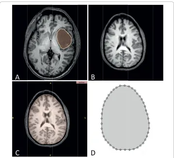
From the two-dimensional contours, the surface and volumetric patches are created using the COMSOL3.3 software (see http://www.comsol.com for details) to represent three-dimensional models of the surfaces and volume of the brain parenchyma and tumor. This software is based on the finite element methods developed for solving partial differential equations, visualization, and meshing and has strong post-processing modules. For creating the 3D model, the slices that are near the craniotomy surfaces have higher resolutions than the slices far from the surface. This means that for each case, we have a specific number of slices with a specific thickness. For the craniotomy surface, we choose more slices than the other parts because if all parts have the same number of slices, the implementation will be time consuming or the accuracy of the model will be insufficient if the total number of slices is small. Therefore, in the craniotomy part, the contours are selected very close to each other and in other parts they are selected relatively far from each other as shown in Figure 2. Also, for the tumor, we use close contours.
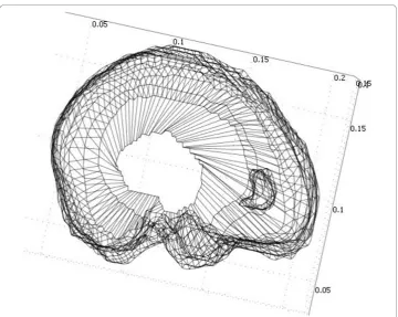
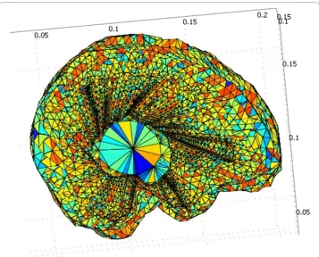
Figure 3 shows the final models of the tumor and the brain such that both volumes can be seen. After creating the 3D models, automatic 4-node tetrahedral meshes with Lagrange shape functions are generated for both of the parenchyma and the tumor using the COMSOL3.3 software. An example of the mesh generated by the software is shown in Figure 4, which consists of 41,617 tetrahedral elements.
Figure 2For creating the 3D model, the slices that are near the craniotomy surfaces have higher resolutions than the slices far from the surface. For the craniotomy surface, we choose more slices than the other parts because if all parts have the same number of slices, the implementation will be time consuming or the accuracy of the model will be insufficient if the total number of slices is small.
Biomechanical Models of Brain
The biomechanical models guided by low-resolution intra-operative images may be used for updating the high-resolution pre-operative images [18,19]. These models can be linear or nonlinear. In our previous work [8], we compared two linear models (elastic and mechanical) and found that the mechanical model generated more accu-rate results. In this paper, we develop a nonlinear model and compare it to the best of the two linear models studied previously, i.e., the mechanical model. Relying on the study of [13], the initial coefficients of the mechanical model are set to Young modules = 3 kPa and Poisson ratio = 0.45. Next, we explain the nonlinear model. The readers are referred to our previous work [8] for the details of the mechanical model.
Non-linear Model
In this model, the brain is supposed to be a single-phase continuum undergoing large deformations. In this analysis, the stresses and strains are measured with respect to the current configuration. Therefore, using Almansi strain and Cauchy stress [20], the vir-tual work principle can be written as:
ij ij iB i
V V
iS i
S
dV=
∫
f u dV+ f u dS∫
∫
, (1)where ij ij V
dV
∫
is the internal virtual work of the strain, f u dViB iV
∫
is the virtualwork of the external force applied to the entire body, f u dSi S
i S
∫
is the virtual work ofthe external force applied to the surface, and uis the displacement parameter. As the brain deforms, the volumeVand surface Sin the integrals of equation (1) change. As such, they are part of the solution and the input data can be used to set their initial values. To find their values after deformation, appropriate finite element procedures can be used to solve equation (1) with equation formula that describes the mechanical property of the material, i.e., appropriate constitutive models. To this end, we use the nonlinear model proposed by [21,22]. This model is suitable for the low strain rates that are typical in surgical procedures and is described in equation (2).
W C g e
d ij k t k n i j N t k = ⎛ − − ⎝ ⎜ ⎜ ⎞ ⎠ ⎟ ⎟ ⎡ ⎣ ⎢ ⎢ ⎤ ⎦ ⎥ ⎥ × − − = + =
∑
∑
∫
{ 0 ( ( )/ )1 1
0
1 1
d
d J J d
i j
[( 1−3) ( 2−3) ]}
(2)
where τkare characteristic times,gk are the relaxation coefficients,Nis the order of
polynomial in strain invariants, andJ1, J2 are strain invariants as described by:
J Trace B J J Trace B
J J B
1
2
3
12 2
2 3 = = − = [ ], [ ] , det (3)
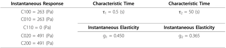
where Bis the left Cauchy-Green strain tensor. We use the stationary form of the equation (2) because we solve the problem for the steady state form of deformation when the deformation of the brain is stabilized. All details about this equation, how their parameters are determined, and how the stationary form of the equation can be found, are described in [22]. The initial values of the model’s parameters are taken from [22] for n = 2, N = 2 as summarized in Table 1.
Boundary Conditions
To solve the equations governing the models, boundary conditions should be specified. To this end, we assume that the exposed surface and the nearby regions are free to move but the remaining surfaces are fixed. The exposed surface is defined manually using the intra-operative images. Thus, the parameteru is free to vary on the exposed
Table 1 Parameters used for the nonlinear model as the initial values for the optimization process
Instantaneous Response Characteristic Time Characteristic Time
C100 = 263 (Pa) τ1= 0.5 (s) τ2= 50 (s)
C010 = 263 (Pa)
C110 = 0 (Pa) Instantaneous Elasticity Instantaneous Elasticity
C020 = 491 (Pa) g1= 0.450 g2= 0.365
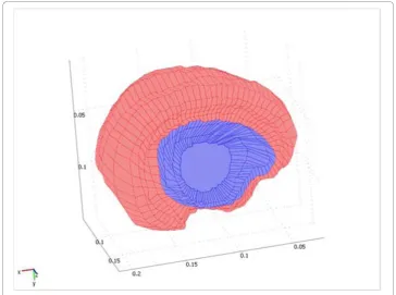
surfaces and the surfaces near it, and is zero on the remaining surfaces. However, it is unconstrained for the inside of the volume. Figure 5 shows the boundary condition for a sample case. The exposed surface is shown in blue and the fixed surface is shown in red. Note that when the skull is exposed, the exposed and the nearby tissues deform.
In both models, we have conditions for the force (F) variable rather than the displa-cement variable. Previous works suggest that this parameter is a constant (fixed) value for each surface and determine its value for each surface by registering the intra- and pre-operative volumes [13]. We fix this parameter for the center of the exposed surface and let it change for the remaining exposed surface. We also useF = ufor the bound-ary conditions of the fixed boundbound-ary nodes because all of the equations lead to the equationKu = F(Kencapsulates all coefficients of the equation) and therefore, accord-ing to [13], the non-diagonal elements of the rigidity matrix Kfor which the deforma-tion is supposed to be known are zero and the diagonal elements are one. Further details can be found in [13].
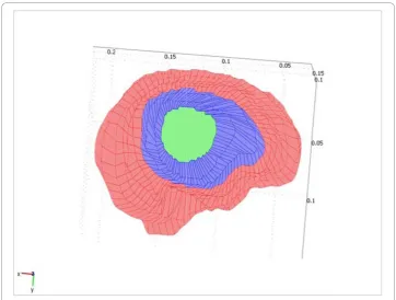
In other words, no forces are applied to the fixed surface so the equivalent force for this surface will be zero. The initial value of the parameter F for the center of the exposed surface is set by examining the MR images of six patients. The exact value of Ffor each part is determined by the optimization process as explained in the next sec-tion. This condition is illustrated in Figure 6. The value of parameterFfor the green surface (the center of the exposed surface) is fixed, for the blue surface (the remaining exposed surface) is unconstrained, and for the red surface (unexposed surface) is zero.
Optimization Process
The parameters of the models change from case to case. Thus, as in our previous work [8], we use approximated parameters as the initial values and optimize them for each case to maximize the accuracy of the results for the known deformations of each case.
As mentioned before, we propose a new approach for determining the parameter F.
The value of this parameter in the center of the exposed surface is also determined in the optimization process. To this end, we choose a cost function defined as the sum of the distances between the actual positions of the anatomical landmarks in the intra-operative images and their corresponding estimated positions based on the deforma-tion results of applying the two models on the pre-operative images.
the optimization process and the other half in the testing process. We use the Maltlab optimization toolbox (fminsearch function) to optimize the cost function and find the optimal values of the parameters as explained next.
In both models, we do not know the exact value of the force applied to the center of the exposed surface of the brain. The value of this parameter determined in sample cases is used as an initial value and the optimal value is determined by the proposed optimization process. In addition, in the mechanical model, the two parameters (Young modulus and Poisson’s ratio) reported in the literature are not the same for different patients and thus they are also optimized for each case. For the nonlinear model, in addition to the initial value for F, the parameters listed in Table 1 are used in the optimization process except the parameters of characteristic time. This is because we study the problem in the steady state which is independent of these para-meters. Also, the parameters g1and g2lead to g1+ g2= g in the equation of the steady state. Therefore, these values are varied to find the minimum error.
Results
Simulation Data
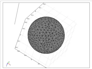
For evaluation of our method, we first apply the models on a brain simulation (a sphere with the diameter of 22 Cm). To model the skull opening, we assume that one section of this sphere is exposed and the other sections are fixed. In the meshing pro-cess, we use 9,028 tetrahedral meshes. Figure 8 shows an example of meshing for the spherical brain model. For each model, we use the brain model with specific para-meters and boundary conditions.
We specify a set of anatomical landmarks for the optimization process and another set for the evaluation of the optimization results. After the optimization, a comparison of the cost function for the evaluation landmarks shows whether the brain deformation is reliably modeled and if the optimization process estimates the model parameters accurately. In this study, we have used 10 points of the sphere for the optimization process and another 10 points for the evaluation of the results. To implement the models, we have used the COMSOL3.3 software which is based on the finite element methods for solving partial differential equations.
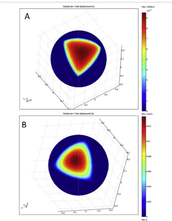
Figure 9 shows the results of the two models for the sphere. Note that deformations of the models are smooth and realistic, similar to those of the brain. This is because
the models solve their equations assuming that the equivalent work applied to a sur-face is zero. Although the results are similar but as we will see next, the results of the nonlinear model are more desirable than those of the other model. For the mechanical and nonlinear models, the mean errors of the points used in the optimization process are 0.1172 mm and 0.0683 mm, respectively. The mean errors of the points not used in the optimization process are 0.2731 mm and 0.1816 mm, respectively. Therefore, accuracy of the nonlinear model is higher than that of the mechanical model. This is because the nonlinear model is more flexible than the linear model. In addition, the number of the parameters of the nonlinear model is larger than that of the mechanical model. Consequently, the nonlinear model fits the landmark data more closely than the mechanical model.
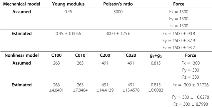
Table 2 shows the assumed and estimated parameters of the two models. As seen, the optimization process estimates the parameters of the nonlinear model more closely than those of the mechanical model. Comparing the final values of the cost function for the points used in the optimization process and those not used in the optimization process, we conclude that the nonlinear model is more appropriate than the linear, mechanical model. However, the execution time of the nonlinear model is six times of the mechanical model. The mean execution time is approximately 35 hours for the lin-ear model and 199 hours for the nonlinlin-ear model for each case. Both models are implemented on a PC with the 1.86 GHz CPU and 4 GB RAM.
Real Data
To evaluate the methods on the real data, we have used six image sets each containing 90 slices with 2.5 mm thickness and 286x286 pixels with 0.86 mm pixel size. Each
Table 2 Assumed and estimated parameters and their variations for the models using a sphere
Mechanical model Young modulus Poisson’s ratio Force
Assumed 0.45 3000 Fx = 1500
Fy = 1500 Fz = 1500
Estimated 0.45 ± 0.0056 3000 ± 175.6 Fx = 1500 ± 90.8 Fy = 1500 ± 87.9 Fz = 1500 ± 93.2
Nonlinear model C100 C010 C200 C020 g1+g2 Force
Assumed 263 263 491 491 0.815 Fx = -300
Fy = 300 Fz = 300
Estimated 263 ±4.0401
263 ±7.8404
491 ±14.4139
491 ±13.4578
0.815 ±0.0083
Fx = -300 ± 9.1726
Fy = 300 ± 10.0278 Fz = 300 ± 8.7998
image set contains both of the pre-operative and intra-operative MRI studies of a brain tumor patient who has undergone surgery.
It is commonly acknowledged that tumors are associated with‘’stiffer’’tissue relative to the normal tissues. However, the volume of a tumor is usually small relative to the volume of the brain. Thus, uncertainties about the tumor’s mechanical properties do not significantly affect the overall displacement field. Consequently, the tumor was simulated using the same constitutive model as‘’healthy’’brain tissue. Also, the para-meters of the two models for the tumor are equal to the brain’s parameters [20]. Of course, if specific model parameters are known for the tumor, they can be used in the proposed algorithm.
Sample results for the mechanical and nonlinear models are presented in Figure 10. The figure shows 3D results for a representative brain where large deformation is shown in red and small deformation is shown in blue. Note that the brain deforma-tions in the two models are smooth. The results indicate that our simuladeforma-tions are realistic.
Figures 11(a)-(b) compare the 2 D contours of the tumor in the coronal sections obtained from the intra-operative images with the results of the optimization process for the two models. Note that the predicted results of nonlinear model show higher levels of matching than those of the linear model. These results show the tumor slices near the craniotomy surface. For the slices deep in the brain or the slices far from the craniotomy, the results of the two models show similar matching; both models follow the deformation quite well. This is because deformations of the brain tissues far from the craniotomy are small.
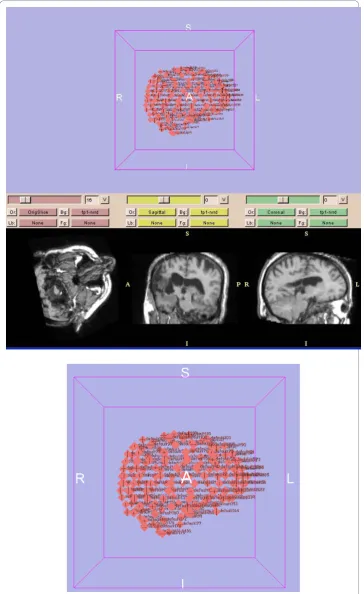
Figure 12 shows the landmark locations estimated by the models and the corre-sponding actual results from the intra-operative images. Note that the points estimated by the nonlinear model (green points) are the closest to the intra-operative points (yel-low points). Also, the points estimated by the linear mechanical model (pink points) are closer to the real results than those estimated by the linear elastic model (the elas-tic model is described in [8]. The numerical values of the maximum and mean errors of the testing landmarks in six cases are presented in Table 3. Table 4 presents the variations of the estimated parameters of the linear and nonlinear models in six cases relative to the initial values. The testing landmarks are mostly near the exposed sur-face. Again, the nonlinear model shows superior performance compared with the linear mechanical model. The errors depend on how much the brain surface is exposed, how much the CSF drains, and in general how much the brain conditions change due to the craniotomy. In addition, the position, the depth, and the size of the tumor affect the results. Finally, selection of landmarks has an important effect on the results; for a conservative evaluation, critical landmarks with relatively large displacements after opening the skull should be considered.
The execution time of the nonlinear model is approximately six times of the linear mechanical model using a personal computer with a 1.86 GHz dual-core CPU and 4 GB RAM. This ratio is an approximation because the execution time depends on the problem complexity, the number of slices, and the mesh resolution that are different for different cases.
parameters of the models can be determined and used in the models to estimate the deformation of the brain without the optimization process.
Conclusion
We have presented a brain shift compensation method based on linear and nonlinear biomechanical models guided by limited intra-operative data. To this end, we have employed finite element methods for descritizing and solving partial differential equa-tions that describe the brain deformation and optimized their parameters for each case for reducing the inaccuracy due to the variations of the parameters from case to case. Also, we have presented a new procedure for defining the force parameter for the models.
To evaluate the proposed method, we have used simulations as well as real MRI data of the brain. Experimental results have shown that both of the linear mechanical and nonlinear models generate shape deformations similar to the brain deformations.
In their applications to a simulation study, the nonlinear model generated the most accurate displacements and the linear mechanical model generated more accurate dis-placements than the linear elastic model. In addition, in their applications to the real data, the nonlinear model generated the best matching for the tumor while the linear mechanical model outperformed the linear elastic model. The landmarks near the exposed surface showed superiority of the nonlinear model based on the maximum and mean error of the surface landmarks not used in the optimization process.
Table 3 Maximum and mean errors for the linear mechanical and nonlinear models
Case 1 Case 2 Case 3 Case 4 Case 5 Case 6
Max error of the mechanical model Δ
Δ Δ x mm y mm z mm = = = 3 0 3 3 . . 1.1 Δ Δ Δ x mm y mm z mm = = = 3 3 3 2 1 0 . . . Δ Δ Δ x mm y mm z mm = = = 3 4 4 4 . . 0.3 Δ Δ Δ x mm y mm z mm = = = 2 9 3 1 . . 0.8 Δ Δ Δ x mm y mm z mm = = = 2 7 2 8 . . 0.4 Δ Δ Δ x mm y mm z mm = = = 4 0 3 4 1 7 . . .
Mean error of the mechanical model Δ
Δ Δ x mm y mm z mm = = = 1 2 1 2 . . 0.4 Δ Δ Δ x mm y mm z mm = = = 1 3 1 0 . . 0.3 Δ Δ Δ x mm y mm z mm = = = 1 3 1 7 . . 0.1 Δ Δ Δ x mm y mm z mm = = = 0 9 1 . .1 0.6 Δ Δ Δ x mm y mm z mm = = =
0 9. 0.8 0.1 Δ Δ Δ x mm y mm z mm = = = 1 0 0 7 . . 0.1
Max error of the nonlinear model Δ
Δ Δ x mm y mm z mm = = = 2 5 3 1 . . 0.3 Δ Δ Δ x mm y mm z mm = = = 3 0 3 1 . . 0.9 Δ Δ Δ x mm y mm z mm = = = 3 2 4 0 . . 0.3 Δ Δ Δ x mm y mm z mm = = = 2 9 2 8 . . 0.7 Δ Δ Δ x mm y mm z mm = = = 2 6 2 4 . . 0.4 Δ Δ Δ x mm y mm z mm = = = 3 0 2 9 . . 1.1
Mean error of the nonlinear model Δ
Δ Δ x mm y mm z mm = = = 0 8 1 1 . . 0.1 Δ Δ Δ x mm y mm z mm = = = 1 2 0 8 . . 0.2 Δ Δ Δ x mm y mm z mm = = = 1 1 1 3 . . 0.1 Δ Δ Δ x mm y mm z mm = = = 0 8 0 9 . . 0.4 Δ Δ Δ x mm y mm z mm = = = 0 7 0 7 . . 0.1 Δ Δ Δ x mm y mm z mm = = = 0 8 0 5 . . 0.9
using anatomical landmarks on the exposed surface of the brain that can be easily measured by the neuro-navigators used in the operation rooms.
Last but not least, the proposed optimization process eliminates the prediction errors due to the variations of the model parameters from patient to patient. It also confirms the conclusion of [23] that the results of the linear and nonlinear model are not con-siderably different and thus, considering the execution speed of the two models, the linear mechanical model may be selected for the modeling of the brain deformation.
Acknowledgements
This work was supported in part by a grant from the University of Tehran, Tehran, Iran. Patient-specific geometric data of the brain used in this work were obtained from the pre- and intra-operative MRI studies of the patients who underwent brain tumor surgery at the Department of Neurosurgery (Harvard Medical School, Boston, Massachusetts, USA) and made available to the authors by the Surgical Planning Laboratory, Brigham and Women’s Hospital (Harvard Medical School, Boston, Massachusetts, USA). The authors gratefully acknowledge and thank Dr. Ron Kikinis and Dr. Tina Kapur for providing this crucial data.
Author details
1Control and Intelligent Processing Center of Excellence (CIPCE), School of Electrical and Computer Engineering,
University of Tehran, Tehran, Iran.2Radiology Image Analysis Lab., Henry Ford Hospital, Detroit, MI 48202, USA.3School of Electrical and Computer Engineering, University of Tehran, Tehran, Iran.4Department of Radiology, Tehran
University of Medical Sciences, Tehran, Iran.
Authors’contributions
HH implemented the algorithms presented in the manuscript, tested the algorithms, and prepared first draft of the manuscript. HS participated in the design and coordination of the study, helped with the testing and evaluation of the proposed methods, and revised the manuscript. RF helped with the implementation and application of the finite element algorithms and evaluation of the simulation results. MG identified the landmarks on the MR images and helped with the evaluation of the clinical results. All authors read and approved the final manuscript.
Competing interests
The authors declare that they have no competing interests.
Received: 2 January 2010 Accepted: 15 September 2010 Published: 15 September 2010
References
1. Chan F, Kassim I, Lo C, Ho CL, Low D, Ang BT, Ng I:Image-guided robotic neurosurgery–an in vitro and in vivo point accuracy evaluation experimental study.Surgical Neurology2009,71:640-648.
2. Hinds O, Polimeni JR, Rajendran N, Balasubramanian M, Amunts K, Zilles K, Schwartz EL, Fischl B, Triantafyllou C: Locating the functional and anatomical boundaries of human primary visual cortex.NeuroImage2009,46:915-922. 3. Tao JX, Hawes-Ebersole S, Baldwin M, Shah S, Erickson RK, Ebersole JS:The accuracy and reliability of 3D CT/MRI
co-registration in planning epilepsy surgery.Clinical Neurophysiology2009,120:748-753.
4. Dumpuri P, Thompson RC, Dawant BM, Cao A, Miga MI:An atlas-based method to compensate for brain shift: Preliminary results.Medical Image Analysis2007,11:128-145.
5. Platenik LA, Miga MI, Roberts DW, Lunn KE, Kennedy FE, Hartov A, Paulsen KD:In vivo quantification of retraction deformation modeling for updated image-guidance during neurosurgery.IEEE Transaction on Biomedical Engineering
2002,49:823-835.
Table 4 Variations of the estimated parameters of the linear mechanical and nonlinear models
Optimized in six cases Model
E 3000 ± 452 Mechanical
ν 0.45 ± 0.03
Resultant Force 91–710
C01 253 ± 45 Nonlinear
C10 253 ± 52
C20 491 ± 73
C02 491 ± 73
g1+g2 0.82 ± 0.03
Resultant Force 121–852
6. Clatz O, Delingette H, Talos IF, Golby AJ, Kikinis R, Jolesz FA, Ayache N, Warfield SK:Robust nonrigid registration to capture brain shift from intraoperative MRI.IEEE Transaction on Medical Imaging2005,24:1417-1427.
7. Bathe KJ:Finite Element Procedures.Prentice Hall, Englewood Cliffs. New Jersey1996.
8. Hamidian H, Soltanian-Zadeh H, Faraji-Dana R, Gity M:Estimating brain deformation during surgery using finite element method: optimization and comparison of two linear models.Journal of Signal Processing Systems2009, 55:157-167.
9. Miga MI, Paulsen KD, Lemery JM, Eisner SD, Hartov A, Kennedy FE, Roberts DW:Model-updated image guidance: initial clinical experiences with gravity-induced brain deformation.IEEE Transaction on Medical Imaging1999, 18:866-874.
10. Lunn KE, Paulsen KD, Liu F, Kennedy FE, Hartov A, Roberts DW:Data-guided brain deformation modeling: evaluation of a 3-D adjoint inversion method in porcine studies.IEEE Transaction on Biomedical Engineering2006,53:1893-1900. 11. Paulsen KD, Miga MI, Roberts DW, Kennedy FE, Platenik LA, Lunn KE, Hartov A:Finite element modeling of tissue
retraction and resection for preoperative neuroimage compension with surgery.Medical Imaging: Visualization, Display, and Image-guided Procedures2001,2:13-21.
12. Miga MI, Sinha TK, Cash DM, Galloway RL, Weil RJ:Cortical surface registration for image-guided neurosurgery using laser-range scanning.IEEE Transaction on Medical Imaging2003,22:973-985.
13. Ferrant M, Nabavi A, Macq B, Black PM, Jolesz FA, Kikinis R, Warfield SK:Serial registration of intraoperative MR images of the brain.Medical Imaging Analysis2002,6:337-359.
14. Ferrant M, Nabavi A, Macq B, Jolesz FA, Kikinis R, Warfield SK:Registration of 3-D intraoperative MR images of the brain using a finite element biomechanical model.IEEE Transaction on Medical Imaging2001,20:1384-1397. 15. Miller K:Method of testing very soft biological tissues in compression.Journal of Biomechanics2005,38:153-158. 16. Miller K:How to test very soft biological tissues in extension?Journal of Biomechanics2001,34:651-657. 17. Miller K, Chinzei K:Mechanical properties of brain tissue in tension.Journal of Biomechanics2002,35:483-490. 18. Clatz O, Sermesant M, Bondiau PY, Delingette H, Warfield SK, Malandain G, Ayache N:Realistic simulation of the 3-D
growth of brain tumors in MR images coupling diffusion with biomechanical deformation.IEEE Transactions on Medical Imaging2005,24:1333-1346.
19. Peña E, Doblaré M:An anisotropic pseudo-elastic approach for modeling Mullins effect in fibrous biological materials.Mechanics Research Communications2009,36:784-790.
20. Wittek A, Miller K, Kikinis R, Warfield SK:Patient-specific model of brain deformation: Application to medical image registration.Journal of Biomechanics2007,40:919-929.
21. Miller K, Chinzei K, Orssengo G, Bednarz P:Mechanical properties of brain tissue in-vivo: experiment and computer simulation.Journal of Biomechanics2000,33:1369-1376.
22. Miller K:Constitutive model of brain tissue suitable for finite element analysis of surgical procedures.Journal of Biomechanics1999,32:531-537.
23. Wittek A, Hawkins T, Miller K:On the unimportance of constitutive models in computing brain deformation for image-guided surgery.Biomechanics and Modeling in Mechanobiology2009,8:77-84.
doi:10.1186/1475-925X-9-51
Cite this article as:Hamidianet al.:Data-guide for brain deformation in surgery: comparison of linear and nonlinear models.BioMedical Engineering OnLine20109:51.
Submit your next manuscript to BioMed Central and take full advantage of:
• Convenient online submission
• Thorough peer review
• No space constraints or color figure charges
• Immediate publication on acceptance
• Inclusion in PubMed, CAS, Scopus and Google Scholar
• Research which is freely available for redistribution