R E S E A R C H A R T I C L E
Open Access
Can the buck always be passed to the
highest level of clustering?
Christian Bottomley
*, Matthew J. Kirby, Steve W. Lindsay and Neal Alexander
Abstract
Background: Clustering commonly affects the uncertainty of parameter estimates in epidemiological studies. Cluster-robust variance estimates (CRVE) are used to construct confidence intervals that account for single-level clustering, and are easily implemented in standard software. When data are clustered at more than one level (e.g. village and household) the level for the CRVE must be chosen. CRVE are consistent when used at the higher level of clustering (village), but since there are fewer clusters at the higher level, and consistency is an asymptotic property, there may be circumstances under which coverage is better from lower- rather than higher-level CRVE. Here we assess the relative importance of adjusting for clustering at the higher and lower level in a logistic regression model.
Methods: We performed a simulation study in which the coverage of 95 % confidence intervals was compared between adjustments at the higher and lower levels.
Results: Confidence intervals adjusted for the higher level of clustering had coverage close to 95 %, even when there were few clusters, provided that the intra-cluster correlation of the predictor was less than 0.5 for models with a single predictor and less than 0.2 for models with multiple predictors.
Conclusions: When there are multiple levels of clustering it is generally preferable to use confidence intervals that account for the highest level of clustering. This only fails if there are few clusters at this level and the intra-cluster correlation of the predictor is high.
Keywords: Clustering, Multilevel, Hierarchical, Sandwich estimator, Robust variance estimate, Logistic regression
Background
Observations are often grouped in assortative clusters, so that two observations from the same cluster tend to be more similar than two selected at random. For example, members of the same household might share genetic and environmental risk factors such that the presence of a dis-ease in one member is predictive of that in others in the same household.
Clustering can influence the amount of uncertainty in parameter estimates. For the sample mean, the standard estimate of the variance must be inflated by a factor 1+ ρ(n−1), where ρis the intra-cluster correlation, which equals the ratio of the variance of cluster means to the total variance of the observations [1], andnis the num-ber of clusters. For measures of association between an outcome(y) and predictor(x)the effect of clustering in
*Correspondence: [email protected]
MRC Tropical Epidemiology Group, London School of Hygiene & Tropical Medicine, Keppel Street, London, UK
the outcome is complicated by the distribution ofxacross clusters—i.e., the degree of clustering inx—and it may not always inflate the variance. In a linear regression model the variance of the regression coefficient associated with the predictor is increased by 1+(n−1)ρxρyrelative to the OLS estimate [2, 3]. Thus clustering has no effect when eitherρx or ρy is zero and a large effect when both are close to one.
Generally, parameter estimates from generalised lin-ear models, such as logistic regression, are consistent in the presence of clustering, provided that the relation-ship between the mean of the outcome and the predictor variables is correctly specified. But the standard vari-ance estimates of the regression parameters that ignore clustering are not consistent, and therefore confidence intervals that are based on these variance estimates are incorrect [4]. Fortunately, it is possible to obtain consis-tent variance estimates for regression parameters using
cluster-robust variance estimates (CRVE), which are con-sistent irrespective of the correlation structure within clusters, provided that observations between clusters are independent [4]. In particular, when there is more than one level of clustering (e.g., individuals clustered in house-holds and househouse-holds clustered in villages), then CRVE applied at the higher level are consistent, despite the correlation structure within the higher-level clusters (vil-lages) being complicated by correlations within the lower-level clusters (households). Thus a researcher who is faced with multiple levels of clustering can obtain consistent confidence intervals by using CRVE at the highest level of clustering: Angrist and Pischke refer to this as ‘passing the clustering buck’ to the higher level [5].
Consistency, however, guarantees lack of bias only asymptotically, i.e., for sufficiently large sample sizes. Unfortunately, CRVE are biased when there are few clus-ters. Furthermore, the bias is usually downward so that confidence intervals are too narrow [6]. There is there-fore a trade-off. At the lower level of clustering there will be more clusters, but observations from different clusters will be dependent. While, at the higher level, observations from different clusters are more likely to be independent but there will be fewer clusters and the CRVE will be biased.
In this study we explore this trade-off in the context of logistic regression. We use a random effects (conditional) model to simulate binary data that are clustered at two lev-els, and fit a marginal model to these data, using CRVE to adjust for clustering at either the higher or the lower level. Before we present the simulation, we describe the rela-tionship between marginal and conditional models, and discuss the intra-cluster correlation as a measure of the degree of clustering.
Methods
Marginal and conditional models
We model the relationship between a binary outcome and a set of binary predictors in the presence of nested clusters, where the disease and predictors can vary in prevalence between clusters. For example, we might want to predict the probability of a disease based on certain risk factors, and the disease and risk factors are known to cluster in households and villages. In this example, house-holds are the lower-level clusters, and they are nested in villages because members of a household belong to the same village.
One approach used to account for clustering is to include random effects in the regression model. For exam-ple, we might model the effects of household and village as independent, normally distributed random variableszjk and uk and include these, together with the predictors x1,. . .,xp, in the model
log
π
ijk
1−πijk
=α0+α1x1ijk+α2x2ijk+. . .+αpxpijk+uk+zjk
(1)
whereπijkis the probability of disease in individualifrom householdjand villagek.
We refer to this as the conditional model as the parame-ter estimates for the predictor variables are conditional on the village and household effects. The model can be fitted by integrating the likelihood over the distribution of the unobserved random effects of village and household, and then maximising this marginal likelihood. A drawback of this approach is that it is necessary to assume distributions for the random effects, and the parameter estimates can be sensitive to the choice of distribution [7].
Alternatively, we can fit a marginal, or population aver-age, logistic regression model that ignores clustering
log
πijk
1−πijk
=β0+β1x1ijk+β2x2ijk+. . .+βpxpijk.
(2)
The parameters of this model can be estimated by fit-ting the model using maximum likelihood, ignoring the cluster effects. This is equivalent to solving a set of esti-mating equations (Eq. A-2 in the Appendix) that have been derived by setting the derivative of the log-likelihood to zero. Each parameter estimates is consistent, provided that the relationship between the probability of disease and predictor variables is correctly specified, but the usual variance estimate based on the second derivative of the log-likelihood is not correct. For a single level of cluster-ing, a cluster robust variance estimate (CRVE) can be used instead (see appendix). This estimate is unbiasedas the number of clusters tends to infinity, but may be biased when the number of clusters is small. When there are mul-tiple levels of clustering, a consistent variance estimate can be obtained by adjusting for clustering at the higher level—this implicitly accounts for lower-level clustering— but, since the number of higher-level clusters is often small, bias maybe a concern.
The parameters, apart from the intercept, represent log odds ratios in both models. But they are interpreted differ-ently in the two models. For example, for a single, binary predictor,x1,β1 is the difference in log odds comparing
individuals withx1=1 andx1=0 across the whole
pop-ulation; whileα1 is the difference comparingx = 1 and
x =0 within a household. The odds ratio, unlike the risk difference and risk ratio, is not collapsible across strata, thereforeα1andβ1will be different unlessα1 = β1 = 0
or there is no variation between households and villages in disease risk.
the random effects model. The parameters of the marginal model are the ‘estimates’ that are obtained when the marginal model is fitted to this dataset. Mathematically, this is equivalent to solving equation A-2 in the appendix, after replacing Yij with Eα[Yij|xij]= πij [8]. Using this approach, Zeger et al. [8] derive the following relationship
β ≈α1+c2σh2+σv2−1/2 (3)
where α is the vector of parameters from the random effects model, β is the vector of parameters from the marginal model and c = 16√3/(15π). From equation 3, it can be seen the odds ratio is closer to the null in the marginal model than the random effects model, and the magnitude of the difference between the odds ratios depends on the amount of variation between clusters, both at the level of the household and the village.
Intra-cluster correlation
The variance of a regression parameter estimate depends on the amount of clustering in both the outcome and the predictor. The intra-cluster correlation, defined as the cor-relation between two observations from the same cluster, can be used to quantify the degree of clustering in both variables. Mathematically, it is defined as
ρ= E(Zij−μ)
Zi∗j−μ
EZij−μ
2 i
∗=i (4)
whereμis the overall mean and the expectation is taken over all clusters and pairs of observations within clusters [1]. Assuming that observations are independent condi-tional on the cluster
ρ= E
μj−μ2
E(Zij−μ)2
(5)
whereμjis the mean for clusterj. Thereforeρrepresents the ratio of the variance in cluster means to the overall variance of the observations.
By definition,ρ = 1 for cluster-level variables because all the variation is then between clusters, butρis less than 1 when variables pertain to lower-level units. For example, in a study where data are collected from different villages, village size would be a cluster-level variable withρ = 1, but for household and individual-level variablesρ < 1. In fact, the intra cluster correlation is usually consider-ably less than 1 for observations made on lower level units. In a survey of binary and continuous outcomes recorded in cluster-based studies conducted in primary care the median intra-cluster correlation was 0.01 and 90 % were less than 0.055 [9].
The intra-cluster correlation of theoutcomecan be cal-culated directly from the random effects model (Eq. 1) for given values of the parameters and covariate. The intra-cluster correlation can also be calculated for each of the
predictors, but in this case since these are not defined by a stochastic model it is calculated based on an empirical ver-sion of Eq. 4. Note that Eq. 5 implies thatρ≥0, but for the predictors the intra-cluster correlation is calculated from the sample rather than the model, consequently the inde-pendence assumption necessary for Eq. 5 is not met and the intra-cluster correlation is not necessarily positive. In fact, it reaches a lower bound of−1/(n− 1) when the prevalence of the predictor is the same in each ofnclusters [3]. We will use the notationρyto denote intra-cluster cor-relation defined by the stochastic model for the outcome andρxˆ to denote the empirical intra-cluster correlation of a predictor.
Simulation
We conducted a simulation study to explore the coverage of confidence intervals for the parameters of the marginal model. The parameter values used in the simulation are given in Table 1, and we estimated coverage for every combination of these parameters.
For each parameter combination, we estimated coverage by simulating 10,000 samples from the population using the conditional model (Eq. 1). The marginal model (Eq. 2) was fitted to each sample, and we calculated confidence intervals unadjusted for clustering (CI(un)), and intervals adjusted for clustering within households (CI(hh)) and vil-lages (CI(vil)). We estimated the coverage for each type of interval by calculating the proportion of the 10,000 inter-vals that contained the true marginal log odds ratio, which was calculated by solving Eq. A-2 in the Appendix with Yijreplaced by Eα[Yij|xij]= πij (see previous section on marginal and conditional models).
We used predictors of the outcome that varied in their degree of clustering within households and villages. At the extremes, we explored predictors where the proportion positive for the predictor was the same in each village such that ρˆx(vil) = −1/(n−1), and predictors where the vil-lage consists entirely of positives or negativesρˆx(vil) = 1. Table 2 shows, for each predictor, the proportion of indi-viduals positive in each village. We used both household, x1−x4, and individual-level,x5−x7predictors. The former
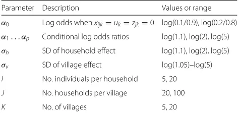
Table 1Parameter values
Parameter Description Values or range
α0 Log odds whenxijk=uk=zjk=0 log(0.1/0.9), log(0.2/0.8)
α1. . . αp Conditional log odds ratios log(1.1), log(2), log(5)
σh SD of household effect log(1.1), log(2), log(5)
σv SD of village effect log(1.05)–log(5) I No. individuals per household 5, 20
J No. households per village 20, 100
Table 2Distribution of predictors (x1-x7) across villages (V1-V5)
and the resulting intra-cluster correlation of the predictor
Proportion of Intra-cluster correlationρˆx(vil) individuals positive
Predictor V1 V2 V3 V4 V5
x1,x5 0.2 0.2 0.2 0.2 0.2 –0.01
x2,x6 0 0.1 0.1 0.3 0.5 0.19
x3,x7 0 0.05 0.1 0.1 0.75 0.48
x4 0 0 0 0 1 1
N.B. In the simulation with 20 villages we created 4 identical sets of villages using the proportions for V1-V5
are the same for all members of the household (e.g., household income) and the latter vary between household members (e.g., age). We fitted models with a single pre-dictor and also multivariable models that included all the predictors simultaneously.
CI(hh) and CI(vil) were calculated using CRVE (see Appendix) with two corrections to adjust for downward
bias. First, the CRVE was inflated by a factor ofn/(n−1), wherenis the number of clusters. Second, the confidence interval was calculated using at-distribution withn−1 degrees of freedom as the reference distribution rather than a standard normal distribution.
We did the simulations in R [10] using the rms package [11] to fit logistic regression models and calculate CRVE.
Results
Simulation results
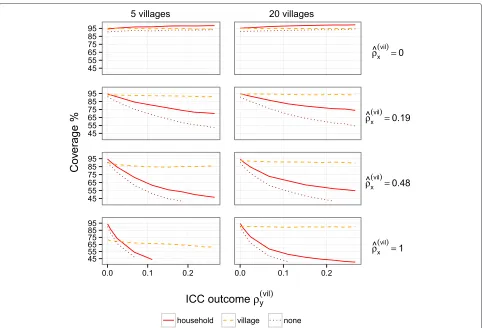
CI(un)and CI(hh) had close to 95 % coverage when there was limited village-level clustering in the outcome or pre-dictor, but for both coverage decreased as clustering in the outcome and predictor increased (Fig. 1). CI(vil) per-formed well when the number of villages was large, and also when the number of villages was small (K =5), pro-vided that the predictor was not too strongly clustered at the village-level. For example, coverage was more than 85 % forρˆx(vil) < 0.5, in models with a single predictor, and in models that included all predictors simultaneously
Fig. 1Coverage of 95 % confidence intervals for the log odds ratio of a household-level predictor. The lines correspond to coverage of confidence intervals that adjust for clustering at the village-level, household-level or do not adjust for clustering. Coverage is presented as a function of the degree of village-level clustering in the outcome as measured by the intra-cluster correlation (ICC). The intra-cluster correlation of the predictor ranges between 0 (top) and 1 (bottom), forK=5 (left) orK=20 (right) villages. The remaining parameter values areα0=log(0.1/0.9),
it was more than 85 % for ρˆx(vil) < 0.2. CI(vil) was only outperformed by CI(hh) when there was limited village-level clustering in the outcome(ρy(vil) < 0.02) and the intra-cluster correlation of the predictor was close to 1 (ρˆ(vil)
x ≈1).
Our findings were similar irrespective of whether a household (Fig. 1) or individual-level predictor (Addi-tional file 1: Figure S1) was used. They were also similar when all predictors (individual and household-level) were included in the model simultaneously (Additional file 2: Figure S2 and Additional file 3: Figure S3), although the coverage of CI(vil)was less good.
Example
We illustrate our findings by analysing data from a ran-domised trial of a house screening intervention to reduce malaria in children 6 months to 10 years [12]. The inter-vention was evaluated in terms of its impact on the numbers of mosquitoes caught, anaemia and malaria par-asitaemia. The study also collected data on risk factors for malaria, including bed net use. Here we will focus on the presence of malaria parasites in the child, and estimate its association with bed net use and house screening. We use data from the six largest villages (or residential blocks in urban areas) collected on 428 children living in 209 house-holds. The protocol was approved by the Health Services and Public Health Research Board of the MRC UK and The Gambia Government and MRC Laboratories Joint Ethics Committee, and the Ethics Advisory Committee of Durham University. All participants provided consent.
At household-level, malaria was strongly clustered, as were the two predictors: the intracluster correlation was 0.47 for malaria, 0.79 for bed net use and 1 for screen-ing (by design). At the village-level, malaria and bed net use were strongly clustered (intra-cluster correlations 0.28 and 0.33), but screening was not clustered because it was randomly allocated to households.
The odds ratio for screening was 1.13 and the 95 % confidence interval adjusted for household clustering was 0.55 to 2.31. Since there are many households and screen-ing is uncorrelated with village, we expect the coverage of CI(hh)to be close to 95 %.
The odds ratio for bed net use was 0.90. The confi-dence interval adjusted for household clustering was 0.50 to 1.63 and adjusted for village clustering it was 0.30 to 2.76. Because malaria and bed net use are both highly clus-tered at the village-level, we expect that CI(vil) will have better coverage than CI(hh).
To further explore the difference between coverage of the two confidence intervals, we fitted a random effects model to the malaria data with bed net use as the pre-dictor. We then simulated samples from this model to estimate the coverage of CI(hh)and CI(vil)for the marginal
odds ratio, using the approach described in the previ-ous section. As predicted, we found that the coverage of CI(hh) (68 %) was considerably worse than CI(vil), which had reasonable coverage (85 %), despite the small number of villages.
Discussion
In general, we recommend using CRVE to adjust for clus-tering at the higher level. From simulation studies, we found that generally the coverage was better when con-fidence intervals were adjusted for the higher level of clustering. Adjusting for the lower level of clustering only gave better coverage (i.e., a higher proportion of confi-dence intervals included the true odds ratio) when the number of higher-level clusters was smalland the intra cluster correlation of the predictor at this level was close to 1. Neither adjustment produced satisfactory coverage when, at the higher level, there were few clusters and the outcome and predictor were both highly correlated with cluster.
We used two simple adjustments to improve the cov-erage of confidence intervals: the variance estimate was multiplied byn/(n−1), and thet-distribution withn−1 degrees of freedom was used as the reference distribu-tion rather than the standard normal distribudistribu-tion. Both adjustments are implemented in the svyset command in Stata. Other methods for adjusting confidence intervals might give better coverage, but are not currently imple-mented in routine software. Pan and Wall [13] suggest modifying the degrees of freedom used for the reference t-distribution, and a number of authors have proposed methods for correcting for the bias in the variance esti-mates [14–16]. Bootstrap methods, in which clusters are resampled with replacement, offer another approach, but do not perform better than CRVE [17].
The results we have presented here are from simula-tion, rather than algebraic demonstration. Nevertheless the simulations cover wide ranges of the key parameters— ρx andρyat the higher level of clustering—and our con-clusions were not sensitive to the values used for the other parameters, except the number of higher level clusters. For this parameter we present results for a small (K = 5) and large (K = 20) number. At K = 20 the cov-erage was close to 95 % when confidence intervals were adjusted for higher-level clustering, and we expect cover-age to improve ifK > 20. We chose not to explore with further granularity the region of parameter space where adjustment at the lower level of clustering is favourable (highρx, lowρyat the higher level of clustering and a small number of clusters at this level) because the region is small and the lower level has only a slight advantage here.
Equations (GEE) this is equivalent to assuming an ‘inde-pendence’ working correlation matrix. The log odds ratio can be estimated more efficiently (i.e., with smaller asymptotic variance) if the correlation structure is used to inform the estimate. For a single level of clustering, a constant correlation between observations from the same cluster is often assumed—the so-called ‘exchangeable’ cor-relation structure. When there are multiple levels of clus-tering one could assume a constant correlation at the higher-level, but this is a crude approximation because the correlation between observations from the same higher-level cluster will depend on whether they also come from the same lower-level cluster. Several authors have there-fore modelled the correlation structure that occurs when there is multi-level clustering and have demonstrated that this gives more efficient estimates compared to either the independence or the exchangeable structure [18–20]. While these methods provide benefit in terms of effi-ciency, the complicated correlation structure is not easily implemented in standard software, and the additional parameters can lead to problems with convergence, par-ticularly when the number of cluster is small [20]. Further-more, the loss of efficiency that results from assuming an independence structure is generally small [4, 21], except when the intra-cluster correlation of the outcome is large (ρy > 0.3) and the predictor varies within clusters [22]. The relative simplicity of assuming an ‘independence’ cor-relation structure (i.e., the CRVE approach discussed in this manuscript) might therefore remain attractive to the applied researcher, even if the resulting estimate it is not the most efficient.
Conclusions
CRVE are commonly used to construct confidence inter-vals that take account of clustering. When clustering occurs at multiple levels, CRVE can be used at the higher level of clustering, except if there are few clusters at this level and the intra-cluster correlation of the predictor is high.
Appendix
In a logistic regression model, the relationship between a binary variableYijand predictorsx1ij,. . .,xpijis
log
πij
1−πij
= β0+β1x1ij+β2x2ij+. . .+βpxpij
= xijβ (A-1)
whereπij=P(Yij=1|xij)for observationifrom clusterj. Assuming responses are independent, the maximum likelihood estimate,βˆ, is the solution to the equations
U(β)= n
j=1
XjYj−πj(β)=0 (A-2)
whereYjis a column vector of responses in clusterj, and Xjis matrix whose columns are the predictors ofYj. Since the Yj are independent, it can be shown by the central limit theorem and using a Taylor expansion that, asymp-totically, as the number of clusters (n) tends to infinity,βˆ is normally distributed with meanβand variance
∂ U ∂β
−1
Var(U(β)) ∂
U ∂β
−1
where Var(U(β)) = jXjVar(Yj)Xj, ∂U
∂β = jXjVjXj andVjis a diagonal matrix with elementsπij(1−πij).
The so-called sandwich estimator, which is also referred to as the cluster robust variance estimate (CRVE), is obtained by replacingπij in Vj with πijˆ and using(yj −
ˆ
πj)(yj− ˆπj)to estimate the covariance matrix Var(Yj).
Additional files
Additional file 1: Figure S1.Coverage of 95 % confidence intervals for the log odds ratio of an individual-level predictor. The intra-cluster correlation of the predictor ranges between 0 (top) and 1 (bottom), for K=5 (left) orK=20 (right) villages. The remaining parameter values are α0=log(0.1/0.9),α1=σh=log(2),I=5,J=20 . (TIFF 30617 kb) Additional file 2: Figure S2.Coverage of 95 % confidence intervals for the log odds ratio of a household-level predictor from a logistic regression model that includes multiple predictors(x1−x7). The intra-cluster correlation of the predictor ranges between 0 (top) and 1 (bottom), for K=5 (left) orK=20 (right) villages. The remaining parameter values are α0=log(0.1/0.9),α1= · · · =α7=σh=log(2),I=5,J=20.
(TIFF 30617 kb)
Additional file 3: Figure S3.Coverage of 95 % confidence intervals for the log odds ratio of an individual-level predictor from a logistic regression model that includes multiple predictors(x1−x7). The intra-cluster correlation of the predictor ranges between 0 (top) and 1 (bottom), for K=5 (left) orK=20 (right) villages. The remaining parameter values are α0=log(0.1/0.9),α1= · · · =α7=σh=log(2),I=5,J=20.
(TIFF 30617 kb)
Abbreviations
CRVE: Cluster robust variance estimate; OLS: Ordinary least squares; CI: Confidence interval; GEE: Generalised estimating equation; SD: Standard deviation.
Competing interests
The authors declare that they have no competing interests.
Authors’ contributions
CB conducted the simulation study. CB and NA wrote the first draft of the manuscript. All authors reviewed the final draft of the manuscript.
Acknowledgements
This work was supported by funding from the United Kingdom Medical Research Council (MRC) and Department for International Development (DFID) (MR/K012126/1). The STOPMAL trial was funded by the UK Medical Research Council and registered as an International Standard Randomised Controlled Trial, number ISRCTN51184253. We would like to thank Richard Hayes for reviewing the manuscript.
References
1. Eldridge SM, Ukoumunne OC, Carlin JB. The intra-cluster correlation coefficient in cluster randomised trials: a review of definitions. Int Stat Rev. 2009;77(3):378–394.
2. Moulton BR. Random group effects and the precision of regression estimates. J Econ. 1986;32(3):385–397.
3. Scott AJ, Holt D. The effect of two-stage sampling on ordinary least squares methods. J Am Stat Assoc. 1982;77(380):848–854.
4. Liang KY, Zeger SL. Longitudinal data analysis using generalized linear models. Biometrika. 1986;73(1):13–22.
5. Angrist JD, Pischke JS. Mostly harmless econometrics. 6 Oxford Street, Woodstock, Oxfordshire OX20 1TW: Princeton University Press; 2009. 6. Bell RM, McCaffrey DF. Bias reduction in standard errors for linear
regression with multi-stage samples. Surv Methodol. 2002;28(2):169–181. 7. Hubbard AE, Ahern J, Fleischer NL, Van der Laan M, Lippman SA, Jewell N, et al. To GEE or not to GEE: comparing population average and mixed models for estimating the associations between neighborhood risk factors and health. Epidemiology. 2010;21(4):467–74.
8. Zeger SL, Liang KY, Albert PS. Models for longitudinal data: a generalized estimating equation approach. Biometrics. 1988;44(4):1049–60. 9. Adams G, Gulliford MC, Ukoumunne OC, Eldridge S, Chinn S, Campbell
MJ. Patterns of intra-cluster correlation from primary care research to inform study design and analysis. J Clin Epidemiol. 2004;57(8):785–94. 10. Core Team. R: A language and environment for statistical computing. R
Foundation for Statistical Computing. Austria: Vienna; 2015. http://www. R-project.org/. Accessed 24 Feb 2016.
11. Harrell FE. rms: Regression Modeling Strategies. R package version 4.4-0. 2015. http://CRAN.R-project.org/package=rms. Accessed 24 Feb 2016. 12. Kirby MJ, Ameh D, Bottomley C, Green C, Jawara M, Milligan PJ, et al. Effect of two different house screening interventions on exposure to malaria vectors and on anaemia in children in The Gambia: a randomised controlled trial. Lancet. 2009;374(9694):998–1009.
13. Pan W, Wall MM. Small-sample adjustments in using the sandwich variance estimator in generalized estimating equations. Stat Med. 2002;21(10):1429–1441.
14. McCaffrey DF, Bell RM. Improved hypothesis testing for coefficients in generalized estimating equations with small samples of clusters. Stat Med. 2006;25(23):4081–4098.
15. Fay MP, Graubard BI. Small-sample adjustments for Wald-type tests using sandwich estimators. Biometrics. 2001;57(4):1198–1206.
16. Mancl LA, DeRouen TA. A covariance estimator for GEE with improved small-sample properties. Biometrics. 2001;57(1):126–134.
17. Cameron AC, Miller DL. A practitioner’s guide to cluster-robust inference. J Hum Resour. 2015;50(2):317–372.
18. Qaqish BF, Liang KY. Marginal models for correlated binary responses with multiple classes and multiple levels of nesting. Biometrics. 1992;48(3):939–50.
19. Chao EC. Structured correlation in models for clustered data. Stat Med. 2006;25(14):2450–68.
20. Stoner JA, Leroux BG, Puumala M. Optimal combination of estimating equations in the analysis of multilevel nested correlated data. Stat Med. 2010;29(4):464–73.
21. McDonald BW. Estimating logistic regression parameters for bivariate binary data. J R Stat Soc Ser B. 1993;55(2):391–397.
22. Fitzmaurice GM. A caveat concerning independence estimating equations with multivariate binary data. Biometrics. 1995;51(1):309–317.
• We accept pre-submission inquiries
• Our selector tool helps you to find the most relevant journal
• We provide round the clock customer support
• Convenient online submission
• Thorough peer review
• Inclusion in PubMed and all major indexing services
• Maximum visibility for your research
Submit your manuscript at www.biomedcentral.com/submit