Volume 19, Number 1, pp. 31–38. http://www.scpe.org
ISSN 1895-1767 c
⃝2018 SCPE
GPU-BASED ACCELERATION OF METHODS BASED ON CLOCK MATCHING METRIC FOR LARGE SCALE 3D SHAPE RETRIEVAL
MOHAMMED BENJELLOUN∗, EL WARDANI DADI†, AND EL MOSTAFA DAOUDI ‡
Abstract. In this paper, we exploit the potential of the GPU in order to accelerate the process of 3D shape retrieval in large databases. Indeed, the massive parallelism of the GPU offers a huge performance in much high-performance computing (HPC) applications. Our solution consists to accelerate the shape matching process of methods that use a specific similarity metric called Clock Matching (CM). This CM measure is used by view-based methods as an efficient solution to compare two 3D models even if they are not presented in same pose and orientation by taking into account all possible poses in the matching phase. However, the increase in the number of comparisons has a strong influence on the execution time. Our challenge is to exploit the maximum benefit of GPU computing resource by considering the difficulty of implementing the CM metric on GPU. Indeed, the descriptor of a given 3D object is organized using a specific data structure (hash table), where only the information whose values are not equal to zero appears in the feature vector, which makes the parallelization on GPU to be not trivial. Experiment results show a reasonable benefit from the GPU approach.
Key words: GPU, 3D Shape retrieval, Clock Matching, CM-BOF, CM-VGG, 3D object.
AMS subject classifications. 68W10, 68P05
1. Introduction. Thanks to the current digitizing and modeling technologies, the number of accessible
and available 3D models on the web is increasing, which yielded large databases of 3D models. This has led to the development of 3D shape retrieval systems [1, 7, 6, 9, 10, 12, 14, 15, 16] that, given a query object, retrieve similar 3D models. These systems work into two essentials phases which are shape indexing and shape matching. The first one consists to compute the descriptor of a given 3D object while the second one, consists to compare the query object with the 3D models in the database. For most of 3D shape retrieval method, the k objects similar to the query are returned until the shape matching is done with the whole 3D objects in the database. When the dataset size gets very large, the shape matching process becomes very challenging. The challenges come especially from the augmentation of computational time.
In order to accelerate the retrieval process, various content-based retrieval methods and approaches have been proposed in the literature [1, 2, 3, 4, 8, 14, 16]. Including sequential solutions [1, 4] and those based on high-performance computing, like multi-core [3]and GPU[2, 8], ... Despite the high-efficiency of HPC solutions, the problem is that there are a few works in the literature that implement the 3D shape retrieval under GPU environment, most of them are partial since they only concern the shape indexing phase [8].
To accelerate the shape matching phase we have already proposed a GPU-based implementation [2], of a given 3D shape retrieval method called BF-SIFT [11]. The solution proposed in [2] is general and it can be applied to several methods based on the same similarity metric which is KLD (Kullback-Leibler divergence), such as Euclidean distance.
In this paper, we propose a GPU-based implementation of a specific similarity metric called Clock Matching (CM). This similarity measure is used by two view-based methods which are CM-BOF proposed by [10], and CM-VGG presented in [14]. The only difference between the two methods is in the way they do shape indexing, the first one uses Bag-Of-Feature [5, 10, 11] while the second one uses the deep learning approach [14]. The CM metric is the common point between them, its basic idea is to compare two 3D objects even if they are presented in different poses and directions by doing a set of comparison according to 24 different poses still exist for a normalized model. This technique permits to overcome the problem of the alignment and the reflexion. However, the increase in the number of comparisons is a very critical point with a strong influence on the execution time.
∗Department of Computer Science, Faculty of Engineering University of Mons, BELGIUM. (mohammed.benjelloun@
umons.ac.be).
†National School of Applied Sciences, LaRi Laboratory, University of Mohammed First, MOROCCO.([email protected]).
Ques-tions, comments, or corrections to this document may be directed to that email address.
‡Faculty of Sciences, LaRi Laboratory, University of Mohammed First, MOROCCO.([email protected]).
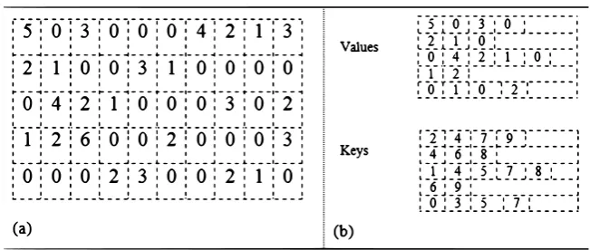
Fig. 1.1.An example of the used two types of data,(a) Indexed structure,(b) Specific structure
Our challenge is to adapt the CM metric to be performed on GPU. Indeed, the difficulty of this implemen-tation is that the feature vector of a given 3D object is organized using a specific data structure cf. Figure 1.1.b, which makes the parallelization GPU to be not trivial. Note that as our contribution concerns not only the CM approach but it resolves the problem of how performing a metric between specific data-structure as a hash table on the GPU.
The rest of the paper is organized as follows. Sect. 2 is devoted to the related works. In Sect. 3 we give a brief description of the Clock matching technique. Our proposed implementation is presented in Sect. 4. Sect. 5 is devoted to the experimental results. We conclude the paper in Sect. 6.
2. Related works. 3D shape content-based retrieval in large datasets is an active research topic related to different fields such as computer vision and pattern recognition,... Indeed, large databases of multimedia data have become available on the web. However, when the dataset size gets very large, the retrieving process becomes very challenging. The challenges come from storage, computation speed, and features representation. Various methods and techniques have been proposed in the literature to accelerate the process of retrieving [1, 2, 3, 4, 8, 14, 16]. The different solutions proposed can be classified into two categories:
• Solutions based on sequential approaches: as an example of these solutions, our proposed work [4], the idea is, for a classified database, we represent each class by a representative in order to orient the process of matching only in the classes of which its representative is the most similar to query. In other work [1], we have proposed an approach that can reduce the number of comparisons of the query in the database.
• Solutions based on high-performance computing(HPC), for multi-core architecture, the idea presented in [3] is to compare the query object simultaneously with P objects, where P is the number of processors. For GPU solutions, Wu [8] have proposed an implementation of SIFT algorithm, this solution is partial because it concerns only a step of shape indexing process and not the shape matching process. To our knowledge, the only work that dealt with the shape matching process on GPU is [2], in which we have proposed a GPU-based implementation of an existing method called BF-SIFT [11]. This solution is general it can be applied to different well-known dissimilarity measurements such as Euclidean L2, Minkowski.
3. Description of the Clock Matching metric. The Clock matching is a specific similarity metric employed for the first time by the CM-BOF [10] method to compare descriptors of two 3D objects. Recently, it’s used in SHREC’17 Track by the CM-VGG method [14]. The CM-BOF and CM-VGG are both view-based methods and the only difference between them is in the way that’s used to characterize the shape of a given 3D object. The first one uses the Bag-Of-Features approach [5, 10, 11] while the second one uses the deep learning approach [14].
in which most of the bins have population zero, and the remaining non-zero elements are small (e.g., <200) positive integers. Thus, the descriptor can be replaced by a lookup into a small table in order to minimize the spatial storage and then the execution time. In this case, a 3D object is described by a matrix of a set of lines, corresponding to each 2D view; while the number of columns differs from one view to another. Each line represents the data structure, it contains the following information: number of non-zero elements, the non-zero elements and its index in the original form cf. Figure 1.1.b.
To compare two 3D objects, the two methods uses the Clock Matching metric. The basic idea of this approach is that, after getting the major axes of an object, instead of completely solving the problem of fixing the exact positions and directions of these three axes to the canonical coordinate frame, all possible poses are taken into account during the shape matching stage. For this, 24 different poses still exist for a normalized model.
When comparing two 3D objects, one is fixed in the original orientation while the second one may appear in 24 different poses. The dissimilarity between two 3D objects is measured by the minimum distance of their all (24) possible matching pairs. The dissimilarity measurement used is:
D(O1,O2)= min
0≤i≤23
N∑v−1
k=0
Dist(dVo1, dVP
i
o2); (3.1)
where O1,O2are the two objects to be compared, Nv is the number of 2D views of a given 3D object. Dist is
the distance between the descriptors of two 2D views and it’s defined as follows:
Dist(dVo1,dVo2)= 1−
∑Nw−1
j=0 min(dVo1(j),dVo2(j))
max(∑Nw−1
j=0 dVo1(j),
∑Nw−1
j=0 dVo2(j))
; (3.2)
where Nwis the number of features in each 2D view. Note that this number differs from one view to another.
4. The proposed implementation. Our solution is to adapt Clock Matching dissimilarity measurements used by CM-BOF and CM-VGG to be performed in the GPU by parallelizing the two functions cf. Eq(3.1) and cf. Eq(3.2) presented in previous section.
In order to maximize the benefits power of GPU computing, by launching the maximum of threads, our general idea is to compare the query object simultaneously with the whole database of 3D models instead of comparing one by one such as the sequential solution.
Launching the maximum of threads using Clock Matching metric is very challenging because this similarity function contains several loops, and it’s necessary to take into account several permutations. The matter is further complicated by the fact that, the data of the descriptors are organized using a specific data structure (cf. Figure 1.1.b) which makes the parallelization GPU to be difficult and not trivial. For example, to compute the following function
N∑w−1
j=0
min(dVo1(j),dVo2(j)),
we need to compute the minimum between elements of two vectors for the same indices, which is not the case because the two vectors are data structured.
To achieve the aim of comparing the query object at the same time as the entire database by launching the maximum of threads, we need a good preparation of the data and an efficient adaptation of the treatment.
Assume that we have a database of m 3D models, and we want to retrieve similar objects for a given query on the GPU. The first step is to prepare the data to be transferred to the GPU. For m 3D objects in the database, the descriptor of each 3D object is represented by a matrix of Nv∗Nw(j), while and Nw(j) is the
size of the jth line; this size is different from one view to another cf. Fig 1.1. All this data will be converted to a one-row vector of size equal m∗Nv ∗Nw(j) and we transfer it to the GPU. We denote this vector by
Regrouping all the data of m 3D objects as one vector will raise the problem of how to determinate the size of each jth line corresponding to each 2D view. To overcome this problem, our idea is to keep the data of the query object in the original form without structuring it. In this case, the query object is represented by a matrix of sizeNw∗Nv whileNw is the size of the descriptor of each 2D view. Since the indexing process of the
object query is performed online, our solution that consists of keeping the initial form permits to reduce the execution time allowed to the structuring process.
So, after transferring the dataDB to GPU, we transfer the data of query object as one vector ofNw∗Nv
which we denotedataQuery.
To perform the shape matching on the GPU, by taking into account the exploiting of the maximum of GPU computing power, our solution consists to separate the treatment of the two functions cf. Eq(3.1) and cf. Eq(3.2) as follows:
• Step 1: we calculate the function ∑Nw−1
j=0 min(dVo1(j),dVo2(j))
• Step 2: we calculate the function max(∑Nw−1
j=0 dVo1(j),
∑Nw−1
j=0 dVo2(j))
• Step 3: we calculate the distance: Dist(dVo1, dVo2)
• Step 4: we calculate the distance: D(O1, O2)
• Step 5: we sort the obtained distance D.
Several kernels are used to calculate the different functions on GPU such as:
1. Kernel 1 is used to compute the minimum between pair of elements of two vectors 2. Kernel 2 is used to compute the maximum between pair of elements of two vectors 3. Kernel 3 is used to compute the sum of elements of a given vector.
4. Kernel 4 is used to compute the division between pair of elements of two vectors
Each step of the five steps has its special adaptation on GPU. To clarify this, we will explain step by step.
4.1. Step 1. For the first step which is∑Nw−1
j=0 min(dVo1(j),dVo2(j)), we use two kernels (kernel 1 and
kernel 2). The first one is to compute the minimum function and the second one to calculate the summation of results obtained by the first kernel.
4.1.1. The minimum function. Instead of computing the minimum between two descriptors one by one and sequentially, our solution is to compute this minimum function simultaneously and in the same time between query and all objects in the database. Our idea is to launch a m*Nv*Nw(j)*24 threads on GPU each
one will execute following instruction:
if(dataQuery[]<dataDB[]) Result[]=dataQuery[ ] else
Result[]=dataDB[]
The problem with launching these numbers of threads simultaneously is how to control access index to vector elements because the size of each row in the database is different from one line to another cf. Figure 1.1. For example, assume we have launched 18 threads to compute the minimum between the two vectors presented in cf. Figure 1.1, for the first four threads there is no problem, each one will execute its instruction as follows:
Thread 1 Thread 2
dataQuery[0]<dataDB[0]) dataQuery[1]<dataDB[1]
Thread 3 Thread 4
dataQuery[2]<dataDB[2]) dataQuery[3]<dataDB[3]
The problem start with the second line of the matrix, it consists of determining the index that permits the access to the second line of query matrix. To overcome this problem our solution is to generate two vectors :
• The first one is to control the acces to information in dataDB, its size is equal to the size of the database data (m∗Nv∗Nw(j) ); we call it T ableSize. Note that as this operation is performed offline. This
For i=0 to m Do For j=0 to NvDo
For k=0 to Nw(j) Do
TableSize[]=j EndFor
EndFor EndFor
• The second one is to control the access to the information in dataQuery, its size is equal to the size of the data query Nv∗Nw. We call itIndexDB.
The two tables are used as follows :
if(dataQuery[ indexDB[j]+Nw*tableSize[i]<dataDB[j])
Result[j]=dataQuery[ indexDB[j] +Nw*tableSize[i]]
else
Result[j]=dataDB[j]
where 0≤i<m*Nv*Nw(j)*24 and 0≤j<m*Nv*Nw(j).
It remains to take into account the 24 permutations possible, to do this our kernel is presented as follows:
global void MinGPU(const int *dataQuery ,const int *indexDB, const int * tableSize, const int *dataDB, const int *Permute, int *ResultMin, int num, int numElements)
{
int i = blockDim.x * blockIdx.x + threadIdx.x; if (i<numElements)
{
int j=i%num;
if( dataQuery[indexDB[j] +Nw * Permute[tableSize[i]]]<dataDB[j] )
ResultMin[i] = dataQuery[indexDB[j] + Nw* Permute[tableSize[i]]];
else
ResultMin[i] = dataDB[j]; }
}
The kernel represented above is not very optimized. To optimize it, we calculate the treatment indexDB[j] + Nw∗tableSize[i] on CPU since it’s an offline operation. To optimize the memory, we transfer the result of this
treatment using the vector allowed to return the result; this vector is called ResultM in. The final kernel is given as follows:
global void MinGPU(const int *dataQuery, const int *dataDB, int *ResultMin, int num, int numElements)
{
int tmp,j;
int i = blockDim.x * blockIdx.x + threadIdx.x; if (i<numElements)
{
j=i%num;
tmp= dataQuery[ResultMin[i]]; if(tmp <dataDB[j] )
ResultMin[i] = tmp ; else
ResultMin[i] = dataDB[j]; }
This kernel is used to executem∗Nv∗Nw(j)∗24 threads simultaneously. The data transferred to GPU memory
for this kernel is as follows:
• The vectordataQuery is of size equal toNw∗Nv
• The vectordataDB is of size equal tom∗Nv∗Nw(j)
• The vectorResultMin is of size equal to 24∗m∗Nv∗Nw(j)
4.1.2. Calculate the sum of the obtained result. In this step we calculate the sum of the sub-vectors of sizeNw(j) of the obtained result (ResultMin). To compute this sum we have used the kernel ‘reduce by key’
of Thrust library by exploitingtableSize vector used previously.
4.2. Step 2. For this step, we proceed as follows:
• We transfer to the GPU the vector that contain the sum of lines of dataDB (∑Nw−1
j=0 dV (j)). Note that
as this sum is calculated offline on the CPU (cf. Figure 4.1). This vector of sizem∗Nv is denoted by SumDB.
• We calculate on GPU of the sum∑Nw−1
j=0 dV (j) of the dataQuery. We obtain by this a vector of size
Nv. We call this vector bySumQuery. Note that as the data of the query is previously transferred to
the GPU memory.
• We calculate the max function simultaneously between the two vectorsSumQuery andSumDB. To do this we proceed as follows : we launch 24∗m∗Nv threads on the GPU, each one will execute the
operation:
tabM ax[i] =max(SumQuery[j], SumDB[P ermute[k] +Nv∗t]), where 0≤i <24∗m∗Nv ,j =i%Nv,
k=i%(24∗Nv) andt=i/(24∗Nv).
To optimize the treatment and the memory by avoiding multiple transferring of data and by avoiding the using of modulo function, The operationP ermute[k] +N v∗tis performed on the CPU, since it’s an offline operation. The corresponding kernel in this case is given as follows:
global void MaxGPU(const int *SumQuery, const int *SumDB,const int *Permute, int *ResultMax, int numElements)
{
int i = blockDim.x * blockIdx.x + threadIdx.x; int j,tmp;
if (i<numElements) {
j=i%66;
tmp= SumDB[ ResultMax[i] ]; if(SumQuery[j]>tmp)
ResultMax[i] = SumQuery[j]; else
ResultMax[i] = tmp; }
}
4.3. Step 3. In this step we use the kernel4 and we launch 24∗m∗Nv threads in order to calculate the
operation : Dist[i] = 66−(ResultM in[i]/ResultM ax[i])
4.4. Step 4. In this step :
• Firstly, we calculate the sum of sub-vector of sizeNvof the obtainedDistvector. This step is performed
on GPU using the kernel 3. We obtain by this a vector of size 24∗m. We call it bySumDist.
Fig. 4.1.calculate the sum of each line of matrices.
100 200 300 400 500 600 700 800
Number of objects
0.0 0.5 1.0 1.5 2.0 2.5
Exe
cu
tio
n t
ime
GPU CPU
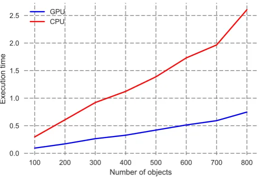
Fig. 5.1.The obtained execution time for different sizes of the database.
4.5. Step 5. In order to return the result, the last step is to sort the obtained vector of distance. This step is performed also on GPU.
5. Experimental results. Tests are performed on a machine with a GPU of type GeForce GT610 of 2048 MB global memory. For the GPU programming, we have used CUDA.
For the 3D object database, we have used Princeton 3D Shape Benchmark database [13]. We have compared between CPU and GPU for the sizes of the database (100, 200, 300, 400, 500, 600, 700, 800).
Figure 5.1, shows the evolution of the execution time of the shape matching process with different sizes of the database and for both implementations on the CPU and on the GPU. The obtained results show that the execution time is significantly reduced for the case of GPU based implementation which means that’s interesting to use this new resource of high-performance computing. On the other hand and always for the case of GPU, the Fig Figure 5.1 shows that the evolution of the execution time when increasing the size of the database is almost linear; if we consider Tm as the GPU time obtained for m 3D objects, the obtained results show as
Tm≈(2∗Tm/2), which means that the large scale can be achieved using GPU. For multi-GPU, the database of
m 3D objects can be divided on the number k of GPUs. Each one performs the matching of m/k 3D models independently.
that use Clock Matching metric. This implementation exploits the maximum of the potential of the GPU and it permits to compare simultaneously, the query object with a large number of 3D models. This has the advantages of obtaining the retrieval results in a very short time, the thing that was well justified by the experimental results. Experimental results show that the execution time is significantly reduced compared to the execution on the CPU. Our proposed solution shows that the large-scale retrieval can be achieved using GPU.
REFERENCES
[1] M. Benjelloun, E. W. Dadi, and E. M. Daoudi,New approach for efficiently retrieving similar 3D models based on reducing the research space. International Journal of Imaging 01/2014; 13(2), pages 104-111.
[2] E. W. Dadi and E. M. Daoudi,GPU-Based for accelerating the BF-SIFT method for large-scale 3D shape retrieval, Multimedia Computing, and Systems (ICMCS), 2014 International Conference on, Marrakech, 2014, pages 38-41.
[3] E. W. Dadi, and E. M. Daoudi.Large Scale 3D Shape Retrieval Based on Multi-core Architectures, Lecture Notes in Computer Science 7853, 2013, pages 295-299.
[4] E. W. Dadi, E. M. Daoudi, and C. Tadonki.Fast 3D shape retrieval method for classified databases, IEEE International Conference on Complex Systems (ICCS) 2012.
[5] J. Fehr, A. Streicher and H. Burkhardt,A Bag of Features Approach for 3D Shape Retrieval, Advances in Visual Com-puting, Lecture Notes in Computer Science, 2009, pages 34-43.
[6] T. A. Funkhouser, M. Kazhdan, P. Min, P. Shilane,Shape-based retrieval and analysis of 3D models, Communications of the ACM - 3d hard copy, Volume 48 Issue 6, June 2005, pages 58-64.
[7] Y. Gao, Q. Dai, M. Wang, N. Zhang,3D model retrieval using weighted bipartite graph matching, Signal Processing: Image Communication Journal Volume 26 Issue 1, January, 2011, pages 39-47.
[8] C. Wu,A GPU Implementation of Scale Invariant Feature Transform (SIFT),http://cs.unc.edu/˜ccwu/siftgpu
[9] A. Koutsoudis, C. Chamzas,3D pottery shape matching using depth map images, Journal of Cultural Heritage, Journal of Cultural Heritage, Volume 12, Issue 2, AprilJune 2011, pages 128-133.
[10] Z. Lian, A. Godil, X. Sun and J. Xiao,CM-BOF: visual similarity-based 3D shape retrieval using Clock Matching and Bag-of-Features, Journal of Machine Vision and Applications; Vol. 24 Issue 8, Nov 2013, p1685 ISBN 0932-8092. [11] R. Ohbuchi, K. Osada, T. Furuya, T. Banno,Salient Local Visual Features for Shape-Based 3D Model Retrieval, IEEE
International Conference on Shape Modeling and Applications (SMI08), Stony Brook University, June 4-6, 2008. [12] L. Pengjie, H. Ma, and A. Ming,Nonrigid 3D model retrieval using multi-scale local features, Proceedings of the 19th ACM
international conference on Multimedia - MM 11, 2011.
[13] P. Shilane, P. Min, M. Kazhdan, and T. A. Funkhouser, The Princeton shape benchmark, in Shape Modeling and Applications Conference, SMI2004, Genova, Italy, June 2004, IEEE, pp. 167178.
[14] M. Savva, F. Yu, H. Su, A.Kanezaki, T. Furuya, R. Ohbuchi, Z. Zhou, R. Yu, S. Bai, X. Bai5, M. Aono, A. Tatsuma, S. Thermos, A. Axenopoulos, G. Th. Papadopoulos, P. Daras, X. Deng, Z. Lian, B. Li, H. Johan, and Y. Lu, S. Mk,SHREC17 Track Large-Scale 3D Shape Retrieval from ShapeNet Core55, Eurographics Workshop on 3D Object Retrieval 2017.
[15] J.W.H. Tangelder and R.C. Veltkamp, A survey of content based 3D shape retrieval methods, Multimedia Tools and Applications, vol. 39, no. 3, pp. 441471, Sept. 2008.
[16] R. C. Veltkamp, G. J. Giezeman, H. Bast, T. Baumbach, T. Furuya, J. Giesen, A. Godil, Z. Lian, R. Ohbuchi, W. Saleem,SHREC10 Track: Large Scale Retrieval, Eurographics Workshop on 3D Object Retrieval 2010.
Edited by: Dana Petcu
Received: Oct 10, 2017