Volume 10, Number 1, pp. 75–86. http://www.scpe.org c 2009 SCPE
MINIMIZATION OF DOWNLOAD TIME VARIANCE IN A DISTRIBUTED VOD SYSTEM∗
ANNE-ELISABETH BAERT†, VINCENT BOUDET†, ALAIN JEAN-MARIE†,AND XAVIER ROCHE†
Abstract. In this paper, we examine the problem of minimizing the variance of the download time in a particular Video on Demand System. This VOD system is based on a Grid Delivery Network which is a hybrid architecture based on P2P and Grid Computing concepts. In this system, videos are divided into blocks and replicated on hosts to decrease the average response time. The purpose of the paper is to study the impact of the block allocation scheme on the variance of the download time. We formulate this as an optimization problem, and show that this problem can be reduced to finding a Steiner System. We analyze different heuristics to solve it in practice, and validate through simulation that a random allocation is quasi-optimal.
Key words: performance evaluation, video on demand, approximation algorithms, constraint optimization problem, simula-tion.
1. Introduction and Problems. This paper is about the replication of data in a particular Grid Delivery Network (GDN). A GDN is a distributed data delivery system that is able to provide video services, among which Video On Demand (VOD). The idea of VOD is to allow users to request video documents at any time, without a preestablished time schedule. One of the main challenge of GDN system resides therefore in ensuring that users can download video at any time with guaranteed, pre-established download time.
The recent literature has pointed out the interest of using distributed systems for massive video distribution [9, 12, 13]. Documents replication and repartition can also solve some performance problems for video distri-bution, and is an effective way to improve the performance of video download time. Those problems have been studied extensively in the literature [2, 13, 10]. Ibaraki et al. employed a replication optimization technique borrowed from the theory of resource allocation problems [5]. Chouet al. gave a comparison of scalability and reliability characteristics of servers by the use of stripping and replication [2].
Venkatasubramanian et. al. proposed a family of heuristic algorithms for dynamic load balancing in a distributed VOD server [10]. Zhou et al. formulate the problem of video replication and placement on a distributed storage cluster as a combinatorial optimization problem [13].
For a popular document, increasing its replication may decrease its download time. However, as the total storage of the system is usually fixed, increasing its replication implies to decrease the replication of other documents. Video replication and placement algorithms based on popularity were therefore developed in [4, 9, 12]. In these algorithms, the most popular videos are all duplicated on the servers, the problem is then to find how much the less popular documents should be replicated. The response waiting time problem is then restricted to certain videos. In [8], the authors analyzed the impact of the division of the documents into blocks on availability and average download time in a general, BitTorrent-like P2P file systems.
As this brief review of the literature shows, there already exist many replication and placement algorithms aimed at optimizing the average download time for videos. However: on the one hand, none of these models applies directly to the GDN architecture, and on the other hand, no attention has been given yet to optimizing the variance (or the standard deviation) of download times. Yet, the system can foresee statistically and guaranteethe download time only if this variance is small. This is the question we address in the present paper. We have shown in a previous work [1] that with an appropriate replication factor, the average download response time is independent of the allocation methods. On the other hand, we showed that the allocation methods have a direct impact on the variance of response waiting time.
The remainder of this paper is structured as follows. In Section 2, we briefly describe the architecture of the system, we also summarize some of the most important differences between GDN and traditional P2P approaches for VOD. In Section 3, we formulate the problem of minimizing the variance of the waiting time as a combinatorial optimization problem called MINVAR. We study this objective function and show the difficulty of this problem. We compute a lower bound on the optimal value for this objective function. In Section 4 we analyze some heuristics to solve the MINVAR problem. We evaluate them in Section 5 our algorithms using extensive simulations representing different situations. Section 6 concludes the paper.
∗This research is supported the French National Agency for the Research, Audiovisual and Multimedia program, project
VOODDO (contract 2007 AM 012-02).
†LIRMM, CNRS, Universit´e de Montpellier 2, 161 rue ADA, 34392 MONTPELLIER Cedex 5, FRANCE. A. Jean-Marie is with
2. Grid Delivery Network description. The system under study is a hybrid architecture based on ideas from P2P Networking and “Grid Computing” called the Grid Delivery Network (GDN). This concept uses the principle of Grid Computing to keep the control of this centralized network. However, to optimize the data transmission and to propose a document delivery network within guaranteed time, this network uses the transport capacity of Peer to Peer networks, through its capacity of multi-source data delivery.
Fig. 2.1.Grid Delivery network’s architecture
The particular GDN system analyzed in this paper is an implementation described in [11] (see also [1]) and represented in Figure 2.1. It is composed of a central server which manages the whole network and hosts which are “partners” of the GDN and deliver the documents to customers. In this GDN, each host is assumed to be a personal computer of the Grid Computing network, which is bound by contract to provide some resources to the system. Nevertheless, hosts are not available all the time to the network; the proportion of time each host is online is denoted withδ.
Documents are divided into pieces called “blocks”, which are distributedand replicated over the partners, in order to improve reliability and decrease response time see Figure 2.2.
Fig. 2.2.Document Delivery in the GDN
The operation of the system is as follows. When some client wants to download a document on the GDN, it first contacts the central server. The server sends a download plan which specifies, for each block of the document, the identity of some host on which the block is stored. The client then executes this plan, by downloading the blocks in parallel from the partners which are online. Then, all missing blocks are downloaded directly from the central server (or some backup data storage).
In [1], we have proposed a probabilistic model of this GDN, and we have shown that, under appropriate assumptions, the download time for a whole document is given by
where N is the number of blocks of the document that happen to be available on the network, and a, b are positive constants.
By replicating a block on several hosts, the GDN increases the probability that some available host owns this block, and therefore that the download time will be smaller. However, as the total hosts capacity of the GDN is limited it is not possible to replicate every document on every host. We have studied in [1] the problem of minimizing theaverage response time, by picking the replication factor of each document appropriately, in function of their popularity, and under memory constraints. We have proved that theaverage download time is independent of the particular way the replicated blocks are assigned to distinct partners. On the other hand, it turns out that this assignment has a very strong impact of the variance of the download time. Since the Quality of Service objective of the GDN is to guarantee the download time to customers, it is important to find assignments which minimize this variance.
3. Response waiting time optimization.
3.1. Variance of the response waiting time. We begin with computing the variance of the download time of a particular document. According to Eq. (2.1), the variance ofRis proportional to the variance of N, on which we concentrate in the remainder.
Let us consider a particular documentD, segmented intoTblocks. LetB1,· · ·, BT be these blocks. Assume that the optimal replication factorLhas been computed so as to optimize the average download time [1]. Define Uj = 1 if the blockBj is available on some online partner, 0 otherwise. Assuming that the hosts’ on-time is uniformly distributed over time, and that hosts are independent, we have:
P(Uj= 1) = 1− L Y
i=1
(1−δ)
= 1−(1−δ)L .
Let N be the number of available blocks of the document D. We haveN =PT
j=1Uj. The variance of N is given by:
Var(N) = T X
j=1
Var(Uj) +X k6=j
Cov(Uk, Uj). (3.1)
We denote byL(j) the list of hosts which own the blockBj. It is known that, using the notation ¯δ= 1−δ, Cov(Uk, Uj) =E(UkUj)−E(Uk)E(Uj)
(3.2) = ¯δ|L(k)∪L(j)|−δ¯|L(k)|+|L(j)|.
The variance ofUj is given by :
Var(Uj) =E(Uj2)−E(Uj)2
(3.3) = ¯δ|L(j)|−δ¯2|L(j)|.
We have :
|L(k)∪L(j)|=|L(j)|+|L(k)| − |L(k)∩L(j)|.
We use the assumption that the replication factor is the same for each block i. e. |L(j)|=L ,∀j, we obtain for Eq. (3.1):
Var(N) =T γ−L(1−γ−L) +γ−2LX k6=j
γ|L(k)∩L(j)|−1
whereγ= (1−δ)−1.
Accordingly, minimizing Eq. (3.1) is equivalent to minimizing the following objective function X
k6=j
3.2. The MINVAR Problem. In this part, we define the MINVAR problem in the language of combi-natorial optimization.
Definition 3.1. Given a bipartite graph G = (T,P,E), where T,P are a set of vertices and E the set of edges, we define the interference function as
J(G, γ) = X b6=b′∈T
γ|L(b)∩L(b′)|, (3.4)
whereL(b)denotes the neighborhood of b. Obviously, the problem does not depend on the nature of the sets T andP but only on their size.
Our problem is the following:
Definition 3.2. The M IN V AR(T, P, L, γ) optimization problem consists in finding one bipartite graph G= (T,P,E)with|T |=T and |P|=P, which minimizes the interference functionJ(G, γ)under constraints
∀b∈ T ,|L(b)|=L . (3.5)
3.3. Complexity of MINVAR. Now, we turn on the complexity of the MINVAR problem.
Definition 3.3 ([3, 7]). A Steiner system S(B, L, P)is a collection of L-subsets (also called blocks) of a P-set such that eachB-tuple of elements of this P-set is contained in a unique block.
We have the following:
Theorem 3.4. There is a Steiner systemS(B, L, P)iff there is a solutionG of theM IN V AR(T, P, L, γ) problem with
T = P!(L−B)!
L!(P−B)! andγ=T(T −1) + 1 (3.6)
that satisfies J(G, γ)< γB. Proof.
If there is a collectionCsolution of the Steiner systemS(B, L, P), then we can assign to each vertexb∈T the neighborhood that matches one of the subsets ofC. There is exactly
P!(L−B)! L!(P−B)!
subsets inC. So each pair (b, b′)∈T2, b6=b′ shares at most (B−1) neighbors. We have created a solutionG
such as
J(G, γ)≤T(T−1)γB−1 < γB.
On the contrary, if there is a solutionG of the MINVAR problem, i. e.,
T =P!(L−B)!
L!(P−B)!, andγ=T(T−1) + 1 (3.7)
withJ(G)< γb then we define a solution ofS(B, L, P) such as the collectionC={L(b)|b∈T}. AsJ(G)< γB, each subset ofP of sizeL appears at most once inC. Furthermore, we have
P!(L−B)! L!(P−B)!
L B
=
P B
then each subset ofP of sizeL appears; we have a Steiner systemS(B, L, P).
Remark 1. In fact, finding the optimal solution of M IN V AR(T, P, L, γ)with T = P!(L−B)!
It is well-known that Steiner systems are very difficult to find. Therefore ProblemM IN V AR(T, P, L, γ) is a complex problem in the general case with no obvious efficient algorithmic solution.
We now provide a lower bound for the interference functionJ(G, γ), which will be useful later to validate solution heuristics.
Theorem 3.5. For every bipartite graphG= (T,P,E)with|T |=T and|P|=P and such that|L(b)|=L for allb∈ T, we have:
J(G, γ) ≥ T(T−1) γ
T2L2/P −T L+q(P−q)/P
T(T−1) , (3.8)
whereq= (T L) mod P.
Proof. We have, using the convexity of the power functionf(x) =γx: J(G, γ)
T(T−1) = X
b6=b′
1 T(T−1)γ
(|L(b)∩L(b′)|)
≥γ(Pb6=b′ T(T1−1)|L(b)∩L(b ′)|)
.
Using the notation1b,p= 1 ifp∈L(b) and 0 otherwise, X
b6=b′∈T
|L(b)∩L(b′)|= X b6=b′∈T
X
p∈P
1b,p1b′,p
=X
p∈P X
b6=b′∈T
1b,p1b′,p
=X
p∈P
δ(p)×(δ(p)−1)
=X
p∈P
δ(p)2−T×L .
The square function is convex and the minimum of X
p∈P
δ(p)2, under constraint X p∈P
δ(p) =T×L ,
is obtained for values ofδ(p) =⌊T L/P⌋or δ(p) =⌈T L/P⌉.
We decomposeT L =P r+q with 1 ≤q < P, and any vector (δ(p))p which components areq times the valuer+ 1 andP−q times the valuer minimizes the function while obeying the constraint. Evaluating the function for such vectors gives the lower bound.
4. Heuristics. In this part, we analyse heuristics to solve M IN V AR(T, P, L, γ) problem. We propose differents algorithms: a greedy algorithm, two algorithms based on the round-robin paradigm, and two based on random choices.
Algorithm 1: Greedy
Data: T,P,Landγ Result: A bipartite graphG
begin
G=∅
fork∈ {1· · ·L}do fori∈ {0· · ·T−1} do
j= arg min j
{J(G ∪(i, j), γ) +J((G ∪(i, j))c), γ)} G=G ∪(i, j)
4.1. Greedy Algorithm. This algorithm begins with an empty graph and, at each iteration, finds the edge which minimizesJ(G, γ) +J(Gc, γ), whereGc is the complementary bipartite graph ofG. It turns out that this algorithm gives better results than a simple greedy algorithm that would minimizeJ(G, γ) at each step. This is illustrated by the example (whereL= 2 andγ= 3) given by Figure 4.1 .
Fig. 4.1.A greedy example forL= 2andγ= 3
Starting from the graph represented with continuous edges, choosing any of the dotted edges gives the same result forJ(G, γ), but only the edge (3,2) minimizesJ(G, γ) +J(Gc, γ). It turns out that this is the only choice towards the optimal solution. MinimizingJ(G, γ) +J(Gc, γ) therefore guides the choice of edges towards better solutions.
4.2. Round-Robin Algorithm. Round-robin algorithms are generally based on a cyclical scan of vertices or edges. We propose two variants.
Algorithm 2: Blocks Round-Robin (BRR)
Data: T,P andL
Result: A bipartite graphG
begin
G=∅;j= 0
fori∈ {0· · ·T−1} do fork∈ {1· · ·L}do
G=G ∪(i, j) ;j=j+ 1 modP end
In this Blocks Round-Robin (BRR) algorithm, we give as neighborhood to each vertex ofT, theL“next” vertices ofP.
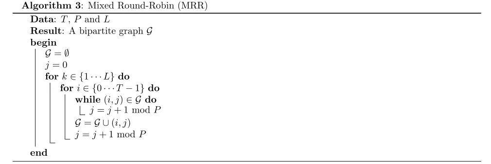
Algorithm 3: Mixed Round-Robin (MRR)
Data: T,P andL
Result: A bipartite graphG
begin
G=∅ j= 0
fork∈ {1· · ·L}do fori∈ {0· · ·T−1} do
In the Mixed Round-Robin (MRR) algorithm, we scan simultaneously the vertices ofT and P, and select the corresponding edge unless it is already in the graph; in that case the corresponding partner is skipped. After Lturns, each vertex ofT has a complete neighborhood.
4.3. Random Algorithms. The RandomSubset algorithm computes for a vertex b its neighborhood of size L among the P possible vertices. It draws uniformly at random one neighborhood among the PL possibilities.
Algorithm 4: RandomSubset
Data: b,P andL
Result: Lvertices from a vertexb begin
S=∅
while|S|< Ldo j=random(1· · ·P) S=S∪(b, j)
end
The Random Algorithm simply performs such a choice, independently, for eachb∈ T.
Algorithm 5: Random
Data: T,P andL
Result: A bipartite graphG
begin
G=∅
forb∈ {0· · ·T−1} do S=RandomSubset(b,P,L) G=G ∪S
end
We show now that it is possible to compute the average value of the objective function for such randomly generated solutions. The key result for this is the distribution of the number of common partners in two neighborhoods.
Theorem 4.1. LetXbb′ =|L(b)∩L(b′)|be the number partners common to both neighborhoods. For every b6=b′, the distribution ofX
bb′ is given by:
P(Xbb′ =k) =
L k
P−L
L−k
P L
and
E(Xbb′) =L
2 P .
Proof. If k elements of P are common between L(b) and L(b′), the set L(b′) is formed by adding L−k
elements chosen among theL−P elements that are not inL(b′) (see the interpretation of the Chu-Vandermonde
convolution in e.g. [6, p. 56]). Hence the formula forP(Xbb′ =k). As a consequence,
E(Xbb′) =
L X
k=0
kP(Xbb′ =k) =
L X
k=0
(L−k) L k
P−L
k P L =L L X k=0 L k
P−L
k P L − L X k=0 k L k
P−L
k
P L
Remark 2. In practical cases, Theorem 4.1 gives us the average number of the blocks in common for a given number of partners in the GDN. For example, if the number of partners is 100 and if L < 10, we can conclude that this number of blocks in common is less than 1 in the GDN.
Corollary 4.2 gives the average value of the objective function for this algorithm.
Corollary 4.2. If G is the graph generated by Algorithm 5, then the average interference function is
E(J(G, γ)) = T(TP−1)
L
L X
k=0 γk
L
k
P−L
L−k
.
If we are convinced that it is possible to find a solution where |L(b)∩L(b′)| ≤ K for each b, b′ ∈ T,
then we may improve the random algorithm : we refuse to accept a neighborhood that has more than K vertices in common with the previous neighborhoods. After N b M ax unsuccessful tries, we increase K to accept neighborhoods more easily.
For example, if we consider 100 partners and the replicationL= 30, we obtain by theorem 4.1 an average intersection of 9. We may want to consider the following constraint: forbid an intersection number greater than K= 5. We come back to the effectiveness of this idea in Section 5.
Thus we obtain the variant fully described in the following Algorithm named Random2.
Algorithm 6: Random2
Data: T,P,L,N b M axandK Result: A bipartite graphG
begin
G=∅
forb∈ {0· · ·T−1}do
OK=false nb=0
while!OK do
S=RandomSubset(b,P,L) OK=true
forb′ ∈ {0· · ·b−1} do if |L(b′)∩S|> K then
OK=false nb=nb+1
if nb > N b maxthen
nb=0 K=K+1 G=G ∪S
end
5. Experimental Evaluation. We proceed now to determine how well these algorithms perform. Since the optimal solution to problem MINVAR is not known, we compare the outcome of the algorithms with an ideal situation given by the theoretical lower bound given in Theorem 3.5. In this section, we describe the experimental settings and then discuss the results.
5.1. General settings. We have built a specific simulator for the heuristics of Section 4. The program implements the three deterministic algorithms, and for the random algorithms, it allows to generate any specified number of independently drawn samples. We have carried out extensive experiments to evaluate the respective performance of the algorithms. In all simulations, we assume γ = 2, which corresponds to an availability of δ= 50% for hosts. The size of documents ranges fromT = 100 to 1000 blocks. The numberP of hosts is 10 or 100, see the figure’s captions.
1 1.05 1.1 1.15 1.2 1.25 1.3 1.35 1.4
100 200 300 400 500 600 700 800 900 1000
Ratio to lower bound
Number of blocks T P=100, L=4, gamma=2
Greedy BRR MRR Random Random2
Fig. 5.1.Algorithms Performance for P=100, L=4
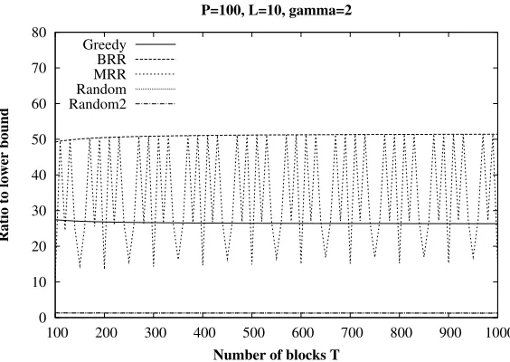
0 10 20 30 40 50 60 70 80
100 200 300 400 500 600 700 800 900 1000
Ratio to lower bound
Number of blocks T P=100, L=10, gamma=2
Greedy BRR MRR Random Random2
Fig. 5.2.Algorithms Performance for P=100, L=10
In real data distribution schemes, these two algorithms are often used because of their simplicity. It is interesting to see that for the present optimization problem, their performance is very far from the lower bound. In addition, the result of MRR appears to suffer sometimes from large fluctuations of arithmetic nature.
Another information is that the performance of the greedy algorithm is very dependent on the data. For some values ofT, its results are better but for some other worst, than the random algorithms. Generally, the algorithm seems to perform well for small L and P parameters. WhenP gets large, the algorithm performs relatively well ifLis small (ex. L= 4), but degrades ifLis larger (ex. L= 10).
The figures also show that the greedy algorithm and the two random algorithms are very close to the lower bound whenLis not too large.
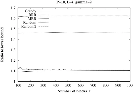
1 1.1 1.2 1.3 1.4 1.5 1.6 1.7
100 200 300 400 500 600 700 800 900 1000
Ratio to lower bound
Number of blocks T P=10, L=4, gamma=2
Greedy BRR MRR Random Random2
Fig. 5.3.Algorithms Performance for P=10, L=4
1.085 1.09 1.095 1.1 1.105 1.11 1.115 1.12 1.125 1.13 1.135
100 200 300 400 500 600 700 800 900 1000
Ratio to lower bound
Number of blocks T P=10, L=4, gamma=2
Greedy Random Random2
Fig. 5.4.Best algorithms comparison
disadvantage for the greedy algorithm is its algorithmic complexity: it isO(P LT3) whereas the complexity of
the random algorithms isO(P LT).
It appears therefore that the random algorithms are the best choice to determine a good block allocation.
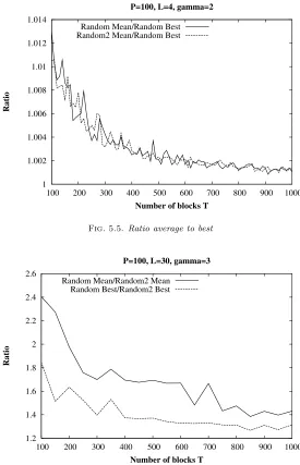
5.3. Analysis of the random algorithm. Focusing now on the random algorithms, we compare in Figure 5.5 the average of the 1000 experiments with thebest allocation found among them. For the Random2 algorithm, we takeN b M ax= 1000.
We observe that the ratio is very close to 1; the standard deviation is actually very small. We conclude that in practice, the first allocation obtained by a random algorithm is probably already close to the optimal solution.
Finally, in Figure 5.6, we compare the Random and Random2 algorithms, through the ratio of their average and best performances.
1 1.002 1.004 1.006 1.008 1.01 1.012 1.014
100 200 300 400 500 600 700 800 900 1000
Ratio
Number of blocks T P=100, L=4, gamma=2
Random Mean/Random Best Random2 Mean/Random Best
Fig. 5.5. Ratio average to best
1.2 1.4 1.6 1.8 2 2.2 2.4 2.6
100 200 300 400 500 600 700 800 900 1000
Ratio
Number of blocks T P=100, L=30, gamma=3
Random Mean/Random2 Mean Random Best/Random2 Best
Fig. 5.6.Random vs Random2 algorithm
the previous neighborhoods turns out to be possible and this improves the block allocation found by 20−40% for a large range of document sizes. For a smaller range of documents size (between 100 and 400), we can say that we obtain an average improvement of 80%.
6. Conclusion and future work. In this paper, we have proposed, and analyzed by simulation, various algorithms for optimizing the variance of download times in a particular distributed architecture, by placing appropriately replications on distributed data servers. In particular, we have shown that conventional Round Robin algorithms do not perform well in general, and that random algorithms are the best practical choice. Our methods have been applied to a real GDN deployment, and we are currently investigating their effectiveness in practice.
REFERENCES
[2] C.-F. Chou, L. Golubchik, and J. C. S. Lui,Striping doesn’t scale: How to achieve scalability for continuous media servers with replication, in Int. Conf. on Distributed Computing Systems, 2000, pp. 64–71.
[3] C. Colbourn and J. Dinitz,The CRC handbook of combinatorial designs, 2nd edition, 2006.
[4] S. Gonzalez, S. Navarro, A. Lopez, and E. L. J. Zapata,A case study of load sharing based on popularity in distributed VoD systems, in IEEE transactions on Multimedia, vol. 8, 2006, pp. 1299–1304.
[5] T. Ibaraki and N. Katoh,Resource allocation problems: algorithmic approaches, MIT Press, Cambridge, MA, USA, 1988. [6] D. Knuth,The art of computer programming Vol. 1, Addison-Wesley, 1973.
[7] F. MacWilliams and N. Sloane,The theory of error-correcting codes, Horth Holland, 1977.
[8] R. Susitaival and S. Aalto,Analyzing the file availability and download time in a P2P file sharing system, in Int. Conf on Next Generation Internet Networks, 2007, pp. 88–95.
[9] K. Tanaka, H. Sakamoto, H. Suzuki, and K. Nishimura,Performance improvements of large-scale video servers by video segment allocation, Syst. Comput. Japan, 35 (2004), pp. 27–35.
[10] N. Venkatasubramanian and S. Ramanathan,Load management in distributed video servers, in Int. Conf. on Distributed Computing Systems, 1997.
[11] VodDNET Company,http://www.voddnet.com.
[12] J. Z. Wang and R. K. Guha,Data allocation algorithms for distributed video servers, in ACM int. conf. on Multimedia, New York, NY, USA, 2000, ACM Press, pp. 456–458.
[13] X. Zhou and C.-Z. Xu,Efficient algorithms of video replication and placement on a cluster of streaming servers, J. Netw. Comput. Appl., 30 (2007), pp. 515–540.
Edited by: Fatos Xhafa, Leonard Barolli Received: September 30, 2008