Volume 7, Number 3, pp. 61–73. http://www.scpe.org c 2006 SWPS
AFPAC: ENFORCING CONSISTENCY DURING THE ADAPTATION OF A PARALLEL COMPONENT
J´ER´EMY BUISSON∗, FRANC¸ OISE ANDR´E†, AND JEAN-LOUIS PAZAT‡
Abstract. Grid architectures are execution environments that are known to be at the same time distributed, parallel, hete-rogeneous and dynamic. While current tools focus solutions for hiding distribution, parallelism and heterogeneity, this approach does not fit well their dynamic aspect. Indeed, if applications are able to adapt themselves to environmental changes, they can benefit from it to achieve better performance. This article presents Afpac, a tool for designing self-adaptable parallel components that can be assembled to build applications for Grid. This model includes the definition of a consistency criterion for the dynamic adaptation of SPMD components. We propose a solution to implement this criterion. It has been evalued using both synthetic and real codes to exhibit the behavior of several proposed strategies.
Key words. dynamic adaptation, consistency, parallel computing
1. Introduction. Grid is an architecture that can be considered as a large-scale federation of pooled resources. Those resources might be processing elements, storage, and so on; they may come from parallel machines, clusters, or any workstation. One of the main properties of Grid architectures is to have variable characteristics even during the lifetime of an application. Resources may come and go; their capacities may vary. Moreover, resources may be allocated then reclaimed and reallocated as applications start and terminate on the Grid. To sum up, Grid is an architecture that is at the same time distributed, parallel, heterogeneous and dynamic. This is why we think distributed assemblies of parallel self-adaptable components is a suitable model for Grid applications.
In our context, we just see the component as a unit that explicitly specifies the services it provides (“provide ports”) and the ones it requires (“use ports”). Required resources are one kind of required services. Service specifications can be qualitative (type specification); they can also be quantitative (quality of the provided or used services). A parallel component is simply a component that encapsulates a parallel code. For example, GridCCM [15] extends CORBA Component Model to support parallel components. A self-adaptable component is a component that is able to modify its behavior depending on the changes of the environment: it may use different algorithms that use services differently and provide different qualities of services. The choice of the algorithm is a component-dependent problem and cannot be solved in a general way at some middleware level. Nevertheless, some generic mechanisms exist in adaptable components that are independent of the component itself. Our research focuses on the design of an adaptation framework for parallel components that provides all those common mechanisms. One of the main problems consists in providing a mechanism for choosing a point in the execution to perform the adaptation in a consistent manner. This article aims at addressing this problem.
Section 2 presents our model of dynamic adaptation for parallel codes to set the context of this article up. Section 3 gives few mathematical definitions that are useful in the remaining text of this paper. Sections 4 and 5 describe how the future of the execution path is predicted to choose the adaptation point at which the adaptation code is inserted. Section 6 discusses the results obtained from our experiments. Section 7 compares our work to others in the area of dynamic adaptation. It also shows similarities with computation steering and fault tolerance. Finally, section 8 concludes this paper and presents some perspectives.
2. Model of self-adaptable components. The dynamic adaptability of a component is its ability to modify itself according to constraints imposed by the execution environment on which it is deployed. It aims at helping the component to give the best performance given its allocated resources. Moreover, it makes the component aware of changes in resource allocation. Resources may be allocated and reclaimed dynamically during the lifetime of the component.
2.1. Structure of a self-adaptable component. With our model of dynamic adaptation Dynaco [3], parallel self-adaptable components can split in several functional boxes (some of them being independent of the
∗IRISA/INSA de Rennes, Campus de Beaulieu, 35042 Rennes, France ([email protected]) †IRISA/Universit´e de Rennes 1, Campus de Beaulieu, 35042 Rennes, France ([email protected]) ‡IRISA/INSA de Rennes, Campus de Beaulieu, 35042 Rennes, France ([email protected])
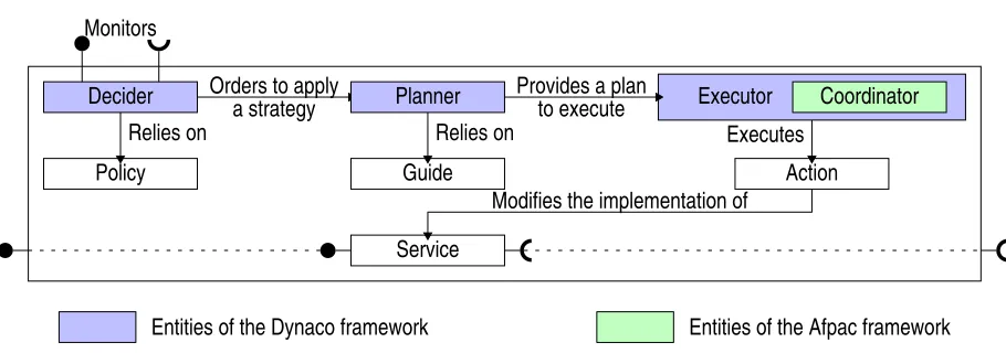
Fig. 2.1.Model of a parallel self-adaptable component
component itself). Figure 2.1 shows the architecture of a parallel self-adaptable component. A short description of the boxes follows.
Themonitors provide the information service about the environment of the component. They should offer two interfaces: a subscription-based event source and a query interface. Monitors are not restricted to collect information about the outside world of the component: the component itself and its activity can be relevantly monitored (for example for estimating its current service rate). Furthermore, nothing prevents the component from being one of its own monitors.
Theserviceof the component is the functionality it provides. The service can be implemented by several algorithms that might be used to solve a single problem. Each of these algorithms uses differently the resources; thus, there is one preferred algorithm for each configuration of the resources allocated to the component.
The actions are the ways to modify the component. They modify the way the service is implemented, replacing the algorithm with another one, adjusting its parameters or anything else. Typically, actions use reflective programming techniques to affect the component.
Astrategyis an indication of the way the component should behave: it states the algorithm that should be executed and the values that its parameters should adopt. Thedecidermakes the decisions about adaptability. It decides when the component should adapt itself and which strategy should be adopted. In order to decide, it relies on the policy and on information provided by monitors. The policy describes component-specific information required to make the decisions. For example, the policy can be an explicit set of rules or the collection of the performance models of the algorithms implemented by the component.
Aplanis a program whose instructions are invocations of actions and control instructions. Thus, plans are programs that modify the component. Theplannerestablishes an adaptation plan that makes the component adopt a given strategy. To do so, it relies on the guide. Theguidegives component-specific information required to build plans. It can consist in predefined plans; or in specifications of how actions can be composed (their preconditions and postconditions for example).
Theexecutoris the virtual machine that interprets plans. In addition to forwarding invocations to actions, it is responsible for concerns such as atomicity of plan execution. The executor embeds a coordinator for synchronizing the execution of the plan with the processes that execute the service. To do so, thecoordinator chooses a point (an instantaneous statement that annotates a special state) within the execution path of the service in order to insert the action.
In the context of parallel components, the service can be implemented either sequentially (exactly one execution thread) or in parallel (several communicating execution threads). In the latter case, the coordinator must implement a parallel algorithm.
Our parallel adaptable components are split in 3 parts. The decider, planner and executor form theDynaco
framework (in blue): they provide the general functionalities of dynamic adaptation. The coordinator is part of theAfpacframework (in green) that is specific to parallel components. Finally, service, actions, policy and guide are specific to the component: they are not included in any framework.
of the provided service. Moreover, for the sake of uniformity, our model abstracts resources as “provide ports” of some component called the environment. The execution environment of a component is thus completely described by the contracts attached to its “use ports”. Consequently, any change in the execution environment is reflected by a change in those contracts, triggering the adaptation.
Contracts are dynamically negotiated and renegotiated: a component negotiates sufficient quality of service with its subcontractors in order to respect the contracts with its clients; it negotiates with its clients the quality of the provided services according to the ones contracted with its subcontractors. In that way, any renegotiation of one contract automatically propagates to the entire assembly of components (the application) to adjust the quality of all the provided services of all components. Consequently, it propagates the trigger of the adaptation to the components that require it.
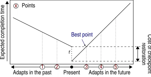
2.3. Performance model. The goal of dynamic adaptation is to help the component to give the best performance. Thus, the model assumes that adaptation occurs when the component runs a non-optimal service given its allocated resources. This means that the completion time is worse than it could be. In a general way, the conceptual performance model of a single-threaded component that adapts itself is shown by figure 2.2. The x-axis is the execution flow of the component with adaptation points labelled from 1 to 5; the curve gives the expected completion time if the component adapts itself at the corresponding point in its execution flow. The lower the expected completion time is for a given adaptation point, the better that adaptation point is.
Fig. 2.2.Conceptual performance model of an adapting component
The adaptation can occur in either the future or the past of the current state. In the case of adapting in the past, it requires the restoration of a checkpoint (that has a costron the curve). At the extremes, adapting in the future is adapting once the execution has ended (or equivalently not adapting at all); while adapting in the past consists in restarting from the begining (purely static adaptation). It appears that whatever the search direction, the best point will always be the nearest one from the current state. In figure 2.2, the best adaptation point is the one labelled 3.
In the case of a parallel component, several curves are superimposed. Because the threads of the component are not necessarily synchronized, the curves are slightly shifted (the present time is not at the same distance of adaptation points for all threads). The global completion time is thus the maximum of the ones for all threads. In this case, the best point can be in the future for some threads and in the past for some others.
In this paper, we arbitrarily chose to consider only the search direction towards the future of the execution. In the case of a parallel component, we look for a global point that belongs to the future of all threads.
2.4. Consistency model. In the case of a parallel service, the coordinator must enforce the consistency of the adaptation. We defined one consistency model, which we called the “same state” consistency model. In this model, the adaptation is said to be consistent if and only if all threads execute the reaction from the same state (this logical synchronization does not require an effective synchronization of the execution threads).
This model only makes sense in the case of SPMD codes (parallel codes for which all threads share the same control flow graph). It has been further discussed in [5].
coordinator to choose an adaptation point. This point is the next one in the future of the execution path. When the threads of the service reach that adaptation point, their control flow is hooked in order to insert the execution of the requested action.
In this paper, we will concentrate on the coordinator. Section 4 describes how the point can be computed; section 5 depicts how an algorithm can be built. In the remaining text of the document, we will call “candidate points” the points at which a reaction can be executed. The one that has been chosen by the coordinator will be called the “adaptation point”.
3. Definitions. This section recalls few definitions about partial orders that are useful in understanding the remaining text of this paper.
Definition 3.1 (poset). A poset (or partially-ordered set) is a pair (P, R) where P is a set and R is a
binary relation overP that is (1) reflexive, (2) antisymmetric and (3) transitive.
(1) ∀x·(x∈P⇒xRx)
(2) ∀x, y· x, y ∈P2⇒((xRy∧yRx)⇒x=y) (3) ∀x, y, z· x, y, z∈P3⇒((xRy∧yRz)⇒xRz)
Definition 3.2 (supremum). Given a poset (P, R), the supremum sup (S)of any subset S ⊂P of P is
the least upper bound uof S inP such that: (1) usucceeds all elements of S and (2)uprecedes any elementv
of P succeeding all elements ofS
(1) ∀x·(x∈S⇒xRu)
(2) ∀v·(v∈P ⇒((∀x·(x∈S⇒xRv))⇒uRv))
Definition 3.3 (infimum). Symmetrically to the supremum, given a poset (P, R), the infimum inf (S) of
any subsetS⊂P of P is the greater lower bound l of S in P such that:
∀x·(x∈S⇒lRx)∧ ∀v·(v∈P ⇒(∀x·(x∈S⇒vRx))⇒vRl)
The infimum ofS in the poset (P, R)is the supremum ofS in P, R−1
.
Definition 3.4 (lattice). A latticeLis a poset (P, R)such that for any pairx, y∈P2, both the supremum
sup ({x, y})and the infimuminf ({x, y}) exist. This defines two internal composition laws:
sup ({x, y}) =x∨y (join) inf ({x, y}) =x∧y (meet)
4. Computing the future. The coordinator needs to find a global point such that it represents the same state for all threads. As it restricts consideration to points in the future of execution paths this point should be the first one in the future for all threads, given the assumption on the performance model depicted in§2.3. 4.1. Local prediction of the next point. For each thread, the coordinator needs to find the next candidate point in the future of the execution path. This point would be the one at which the coordinator is going to execute the reaction in the case of a single-threaded component.
4.1.1. General schema. An execution path can be seen as a path in the control flow graph that models the code. If loops are unrolled (for example by tagging nodes with indices in iteration spaces), the control flow graph defines a “precedes” partial order between the points of a code. Given this relation, each thread of the parallel component is able to locally predict its next point at least in trivial cases, when no conditional instruction is encountered (in this case, nodes in the control flow graph have at most one successor).
4.1.2. Uncertain predictions. In the general case, predicting the future of an execution path is undeci-dable due to conditional instructions: their behavior is unpredictable since it depends on runtime computations. This occurs for both conditions and loops, which appear as nodes having several successors in the control flow graph.
• Postpone. The computation of the adaptation point can be postponed until the effective behavior of the instruction is known. Once the unpredictable instruction has been executed, the computation of the adaptation point resumes with a new start point (the one that is being entered).
• Skip. The computation of the point can move forward in the control flow graph until all control subflows merge. In this case, the prediction jumps over loops and conditions.
• Force. The behavior of the conditional instruction can be guessed when additional static information is available. With this strategy, one branch of the conditional instruction is assumed accordingly to some application-dependent knowledge; then some application-level mechanism enforces that the execution path respects this assumption.
Two examples that follow illustrate the usage of the “force” strategy. Firstly, it is possible for some loops to insert unexpected empty iterations; in this case, it can be guessed that the conditional instruction will execute the branch that stays in the loop; this behavior can be enforced by making one more empty iteration on-demand. Secondly, if the code includes assertions to detect error cases, it could be reasonably assumed that those assertions hold; in this case, it can be guessed that the corresponding conditional instruction will execute the branch leading to error-free cases. As mispredictions exactly match detected runtime errors, error handlers invoked upon assertion failures can be used to handle effects of mispredictions.
The above examples exhibit two interpretations of the “force” strategy. In the first example, the coordinator changes the execution behavior of the component in order to fit its requirements. The coordinator uses the static knowledge about the component to ensure that this change does not have any semantic impact on produced results. In the second example, the coordinator let the component execute its normal behavior and simply exploits static knowledge to make its prediction.
4.2. Characterization of the chosen global point. The point that should be chosen is the supremum u, if it exists, of the set S of the next local points for each thread with respect to the “precedes” partial order (noted ). Indeed, the property ∀x·(x∈S⇒xu) guarantees that u is in the future of all threads; the property∀v·(v∈P ⇒((∀x·(x∈S⇒xv))⇒uv)) means thatuis the first point amongst those in the future of all threads.
Even if loops are unrolled, the control flow graph is not a lattice as it may contain patterns such as the one of figure 4.1(a). In this example, the supremum sup ({P1, P2}) does not exist. This pattern captures a subset of conditional instructions. The three strategies that has been identified for locally predicting the next point can be used to work-around non-existence of the supremum.
• Postpone. Postponing the computation of the adaptation point until the unpredictable instruction has been executed can be seen as inserting a special node that models that instruction in the control flow graph. For example, in figure 4.1(b), a node C has been inserted to represent the conditional instruction. When such a node is chosen, a new round for finding a satisfying point is started once the corresponding instruction has been executed.
• Skip. Skiping the conditional block is equivalent to compute the supremum within the subset defined by:
{a|∀y·((∀x·(x∈S⇒xy))⇒(ay)∨(ya))}
This set contains the points that are related to all successors of all points in S. Those points are guaranteed to be traversed by any execution thread starting from any point inS. The definition of that set ensures that upper bounds ofS in that set are totally ordered by . Consequently, the supremum ofSin that set ordered byexists if at least one upper bound exists. In the given example, it restricts to compute the supremum sup ({P1, P2}) in{P1, P2, P5}; this supremum exists.
• Force. Forcing one branch of a conditional instruction removes all out edges but one of the correspon-ding node. This is sufficient to make the supremum exist. For example, on figure 4.1(c), the conditional instruction that followsP1 has been forced such that it always leads toP3.
(a) Pattern which prevents the supremum from existing
(b) Inserting nodes for conditionals
(c) Removing branches of conditionals
Fig. 4.1.Example of control flow graph with non-existent supremum
5. Building an algorithm. In order to solve the problem of finding a point in the case of a parallel service, an algorithm has been designed.
5.1. Identification of the candidate points. Having a good identification system for the points is a key issue. Indeed, as§4.2 has shown, the case of parallel self-adaptable components requires the computation of the supremum of a set of points. This requires to be able to compare easily candidate points with respect to the “precedes” partial order. However, with naive point identification, deciding whether a candidate point precedes, succeeds, or is not related to another one requires the computation of the transitive closure of the control flow graph with unrolled loops. The same apply for the join composition law. This is why a smarter identification system for the points is needed.
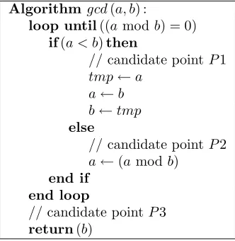
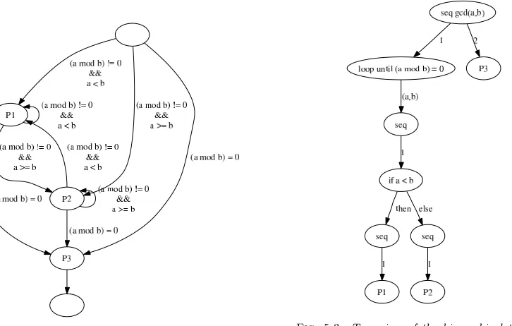
5.1.1. Description of the identification system. We think that the good representation to use is a tree view of the hierarchical task graph. Figure 5.1 gives an example algorithm that has been annotated with candidate points; figure 5.2 shows the control flow graph between annotated points; figure 5.3 shows the corresponding tree view. The edges of the tree are labelled as follows:
• out edges of loop nodes are labelled with the value of the indice within the iteration space of the loop;
• out edges of condition nodes are labelled with either the symbol “then” (the condition is true) or the symbol “else” (the condition is false);
• other edges (out edges of block nodes) are labelled with the execution order number in the control flow.
Algorithm gcd(a, b) :
loop until((amodb) = 0) if(a < b)then
//candidate pointP1 tmp←a
a←b b←tmp else
//candidate pointP2 a←(amodb) end if
end loop
//candidate pointP3 return(b)
Fig. 5.1.An examplary algorithm
Fig. 5.2.Control flow graph of the algorithm 5.1
Fig. 5.3. Tree view of the hierarchical task graph of the algorithm 5.1
the edges traversed by the path from the root to the leaf corresponding to it. For example, the node “P3” is identified byh2i; the node “P1” is identified by the sequenceh1,(a, b),1,else,1i.
5.1.2. Order on points. The set of edge labels in the tree isE=N∪I ∪{then, else}, whereNis the set of execution order numbers (natural numbers) andIthe iteration space partially ordered by an application-specific relationI. We define the following partial order over the setE of edge labels of the tree:
∀x, y· x, y ∈ E2
⇒ xE y⇔ x, y∈N2∧x≤y∨ x, y∈ I2∧xI y
Notably, the two constants “then” and “else” are set not comparable to other values and values in iteration spaces (such as (a, b) in the example) are partially ordered by an application-specific relation.
The edges of the control flow graph (that represent the “precedes” partial order between points) are (gra-phically) transverse to those of the tree. Consequently, the lexicographical partial ordern
E on the sequences
is equivalent to the partial order on points defined by the control flow graph. Thus, with this identification system, deciding whether a point precedes, succeeds, or is not related to another one can be computed as a direct lexicographical comparison (not requiring the computation of the transitive closure of the control flow graph anymore). Moreover, this ordering directly takes into account the loop indices in iteration spaces, whereas the control flow graph does not.
5.1.3. Discussion. This identification system makes sense only in the case of a parallel component in which all threads are allowed to have different dynamic behaviors (different behavior of conditionnal instructions and loop indices desynchronization). Otherwise, a simple counting identification system is sufficient. Furthermore, in the case of a non-parallel component, no identification system is required.
In the above description of the identification system, in the tree view of the hierarchical task graph, leaves are candidate points and internal nodes are “sequence”, “loop” and “if” control structures. This restricts the expressivity for writing programs. Function calls can be represented as leaves that connect to the root the target function tree, as long as the function is bound statically. Thanks to that connection, the sequence identifying a point includes the complete call stack used to reach that point. Problems arise with runtime function binding upon calls (for example calls through pointers) and with “goto” like instructions. In those cases, the proposed order relation does not respect the control flow graph. As programs can be rewritten in order to respect those restrictions, further discussion about control structures is beyond the scope of this paper.
this point simply consists in following the edges of the control flow graph. This corresponds to a depth-first traversal of the tree from the left to the right. This traversal begins at a start point that is at least the one being executed at the time of the computation.
5.3. Instrumentation of the code. In order to predict the next candidate point in the future of the execution path, the coordinator must be able to locate the actual execution progress in the space of the candidate points. As it must be able to build the sequence identifying the candidate point that is being executed by the execution thread, the coordinator requires an instrumentation of the code.
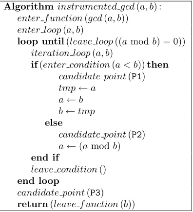
The instrumentation of the code consists in inserting some pieces of code at each node of the tree view of the hierarchical task graph as presented at the preceding section. The figure 5.4 shows an example of an instrumented algorithm.
Algorithm instrumented gcd(a, b) : enter f unction(gcd(a, b)) enter loop(a, b)
loop until(leave loop((amodb) = 0)) iteration loop(a, b)
if(enter condition(a < b))then candidate point(P1) tmp←a
a←b b←tmp else
candidate point(P2) a←(amodb) end if
leave condition() end loop
candidate point(P3) return(leave f unction(b))
Fig. 5.4. Instrumented version of the algorithm 5.1
The process of inserting the instrumentation statements in the source code of the component can be largely automated using aspect-oriented programming (AOP [13]) techniques. We have proposed in [18] a static aspect weaver whose join points are the control structures. This weaver has been successfully used to insert the instrumentation statements. It relies on candidate points, which are placed by hand by the developer, to detect which control structures need to be instrumented (those that contain at least one candidate point).
5.4. Protocol for computing the supremum. Many trivial protocols might be designed to compute this supremum (for example, centralized). Many already exist to compute a maximum (in particular for leader election); they can easily be modified to compute a supremum instead of a maximum. However, we think that a specific protocol suits better this case.
5.4.1. Motivation for designing a specific protocol. The full set of the local adaptation points is not always necessary to compute the supremum. The idea is to superimpose the agreement protocol and the local computations of the next candidate point in order to exempt some of the execution threads from computing their local adaptation point. In particular, it is interesting to exempt those whose prediction is postponed due to conditional instructions. Indeed, it allows the computation of the local adaptation point to resume sooner with a start point that is further in the execution path. Moreover, superimposing the protocol and the computation evicts the earliest adaptation points sooner than if the whole set of local adaptation points must be computed. This avoids situations in which the execution thread tries to execute through a locally chosen point that has not been either confirmed or evicted yet.
give clues to the other threads. These clues can be for example the root node of the subtree representing the conditional block. When a thread receives a proposition or a clue, it may take different actions depending on how it compares to its own proposition.
• If its own proposition is better (that is to say in the future of the received one), it rejects the received proposition.
• If the received one is better, it is adopted.
• If the two propositions are not comparable, the thread retracts its proposition and computes a new one that takes into account the two previous ones. The computation starts at the point at which the control subflows merge (the supremum of the two points).
• If both propositions are the same, the thread agrees with the sending thread.
The protocol also progresses when an execution thread provides new information. For example when the functional thread executes a conditional instruction, it may retract its clue and propose some new information. The protocol ends when all threads agree with each other’s and when the agreement is on a true proposition (not just a clue). This means that they all have adopted the same point.
5.4.3. Anatomy of the protocol. We have designed a specific protocol to solve this problem. This protocol is based on a unidirectional ring communication scheme. Each thread confronts its proposition with the one of its predecessor and sends it only to its successor in the ring. The end of the protocol, namely the reach of the agreement, is detected using a Dijkstra [6]-like termination algorithm. Our protocol distinguishes strong propositions (values that can be chosen by the agreement) from weak propositions (values that forbid the agreement to conclude, previously called clues). The protocol allows threads to retract their proposition. It strictly defines the criteria of the consistency of retraction.
Our protocol is pessimistic. If an execution thread tries to get through a point thought to be the chosen one, the algorithm refuses to speculate whether it should allow the execution thread to continue or execute the reaction. It rather suspends the execution thread until it gets certainty. As a result, because the “postpone” strategy eases such situations (as described in§4.3), this strategy tends to increase the risk of suspending the execution thread.
6. Experiments. The experiments presented here aim at comparing the strategies described at § 4.1.2 with regard to functional code suspension and delay before the execution of the reaction. The goal is to exhibit and validate the expected behaviors described in§4.3. This characterization would help developers to choose the right strategy depending on their code.
Three experiments have been made: synthetic loop code, synthetic condition code and NAS Parallel Bench-mark 3.1 [14] FFT code. Only the results of the latter will be presented and discussed.
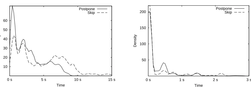
6.1. Experimental protocol. The experimental protocol consists in trigerring adaptation many times at random intervals (with uniform distribution to avoid implicit synchronization between the functional code and the adaptation trigger) while the code is being executed by a 4 processors cluster. Experiments result in two data series: one indicates for each adaptation the time elapsed between the trigger and the effective execution of the reaction; the other gives the time during which the functional thread has been suspended while choosing the point at which to adapt. For each data series, one curve is drawn that gives an approximate measure of the density of samples for each observed value.
6.2. Observations. Figures 6.1 and 6.2 show the results with the FFT code. This experiment aims at comparing the “postpone” and “skip” strategies for conditional instructions within a main loop. The main loop has the “force” strategy so that the synchronization and communication statements induced by our algorithm are exclusively related to the inner instructions. This prevents distortions of the observations.
Figure 6.1 shows that the “postpone” strategy tends to select an adaptation point that arrives sooner in the execution path than the “skip” strategy. Conversly, figure 6.2 shows that the “postpone” strategy tends to suspend the functional code for a longer time than the “skip” strategy. Indeed, the “postpone” strategy leads to higher density of samples up to about 0.5 s of functional code suspension. However, this observation has to be balanced as it appears that both strategies do not suspend the functional code in most of the samples.
60
50
40
30
20
10
0 s 5 s 10 s 15 s
Density
Time
Postpone Skip
Fig. 6.1.Density curve for adaptation delay
200
150
100
50
0 s 1 s 2 s 3 s
Density
Time
Postpone Skip
Fig. 6.2.Density curve for suspension time
The observations are explained by the fact that the “postpone” strategy tends to delay the agreement in order to choose a more precise point (closer to the current state), in comparision to the “skip” strategy. It makes the “postpone” strategy increase the risk for other threads to reach that point before the agreement is made, and thus to suspend their execution. On the other side, the “skip” strategy tends to choose a point that is further in the future of the execution path; it results in a lower risk for other threads to reach that point before the agreement is made and thus to suspend their execution.
Consequently, if the time between a conditional instruction and the following point is large enough to balance the delay of the agreement, the “postpone” strategy should be preferred as it results in a sooner adaptation. Otherwise, the “skip” strategy should be used in order to avoid the suspension of the execution thread.
7. Related works and domains.
7.1. Other projects on dynamic adaptation of parallel codes. Most of the projects that faced the problem of dynamic adaptation such as DART [16] do not consider parallelism. Other projects such as SaNS [8] and GrADSolve [17] build adaptive components for Grid. Those projects target adaptation only at the time of component invocation. This supposes a fine-grain encapsulation in components; otherwise, if methods are too long, adaptation is defeated because it cannot occur during execution. Within the context of Commercial-Off-The-Shelf (COTS) component concept, sufficiently fine-grained encapsulation for the dynamic adaptation to make sense only at invocation level does not appear valuable enough; whereas sufficiently coarse-grained encapsulation for valuable COTS components are not able to really dynamically adapt themselves if they do so only at each invocation. This is why we think that components should be able to adapt themselves not only at method calls, but also during the execution of methods.
The Grid.It project [2] also faces the problem of dynamically adapting parallel components. The followed approach is based on structured parallelism provided by high-level languages. The compiler generates code for virtual processes that are mapped to processing elements at run-time. An adaptation consists in dynamically modifying this mapping. This adaptation can be done within language constructs transparently to the deve-lopper. In this case, the consistency enforcement mechanism can rely on assumptions on the overall structure of the program as it is generated by a compiler.
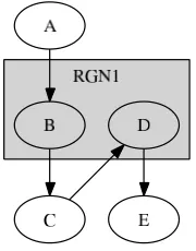
Fig. 7.1. Example of a region in a PCL static task graph
schedule the reaction at the C → D edge for both threads (our “same state” consistency). One solution might be to put B and D in two different regions; but in this case, PCL fails specifying that the reaction can be scheduled either before B or before D, but at the same edge for all threads. Furthermore, PCL is unable to handle the case of thread desynchronization in loops (one thread doing more iterations than ano-ther does) for regions being in such a loop. The simple region counter is not sufficient to solve this pro-blem.
7.2. Resource management in Grid infrastructures. The dynamic characteristic of Grid architecture appears well accepted, as reflected by the presence of monitoring services such as Globus MDS. On the other side, job management usually considers that the set of resources allocated to one job remains constant for the whole lifetime of the job. Approaches such as AppLeS [4] and GridWay [12] show that even Grid applications can benefit from non-constant schedules. With those two projects, when the scheduler or the application detects that a better schedule can be found, the application checkpoints itself, then the job is cancelled and resubmitted with new resource constraints. Our approach is slightly different. We assume that the resource management system is able to modify job schedules without having to cancel and resubmit jobs. Thanks to this assumption, checkpointing and restarting the application is not required, potentially leading to lower cost for the adaptation in particular when the intersection before and after the rescheduling is not empty.
7.3. Computation steering. The problem of steering a parallel component is very close to our problem of adapting this component. Indeed, in both cases, we need to insert dynamically code at some global state. The EPSN project [10] aims at building a platform for online steering and visualization of numerical simula-tions. In [11], the authors describe the infrastructure they built to do the steering. Their structured dates is similar to our candidate point identification system. Both systems are based on similar representations of the code. Moreover, steering like dynamic adaptation tries to find the next candidate point in the future of the execution path. Thus, computation steering and dynamic adaptation may benefit from fusionning in a single framework.
7.4. Fault tolerance. Fault tolerance might be seen as a particular case of dynamic adaptation. Indeed, it is the adaptation to the “crash” of some of the allocated resources. However, things are not that simple. Fault tolerance encompasses two different problems: the recovery of the fault and the adaptation to the new situation. Only the second one really belongs to the problem of dynamic adaptation. Many strategies can be used to recover from faults. The closest one from dynamic adaptation is probably checkpointing in the sense it requires some global points. Whereas dynamic adaptation can look for a point in the future of the execution path, checkpointing requires a point in the past. Nevertheless, mechanisms required by dynamic adaptation may be useful to implement recovery strategies based on checkpointing. The instrumentation of the code can be used as hooks at which checkpoints can be taken. Indeed, it implicitly statically coordinates the checkpoints of all threads, avoiding the problem of computing a global consistent state. Reciprocally, dynamic adaptation can take advantage of the techniques that have been developped to checkpoint and restart computations in the area of fault-tolerance.
8. Conclusion. In this paper, we have briefly described the overall model we introduced to build self-adaptable parallel components. This paper essentially focuses on the coordinator functional box of theAfpac
The protocol we designed follows a pessimistic approach with regard to the fact that the execution thread may go through a confirmed point. In the future of our work, we will study how optimistic approaches can be designed. For example, when the functional code reaches a point suspected to be chosen but not yet confirmed, it may continue its execution instead of waiting for the point to be either confirmed or evicted. If at the end that point is confirmed, the situation may be repaired by rolling-back the functional code.
Moreover, our coordinator searches adaptation points exclusively in the future of the execution path. Ho-wever, this is an arbitrary choice that has no other justification than simplifying algorithms. In our upcoming researches, we will study how algorithms can be generalized in order to allow the coordinator to look for adap-tation points in in both directions (future and past). Thanks to this, chosen adapadap-tation points may be closer to the optimum.
Finally, our “same state” consistency model has to be extended to the case of non-SPMD components: we have already thought of another consistency model defined by a customizable correspondence relation between the candidate points of the threads.
As a longer term research, we are working on completing our architecture in order to build a complete platform. In particular, we are studying how generic engines can be used within ourDynacoframework. We are also investigating protocols for adaptation within assemblies of components. Endly, we are studying how a resource manager could take advantage of applications able to adapt themselves.
Acknowledgement. Experiments described in this paper have been done with the Grid 5000 French testbedhttp://www.grid5000.fr/
REFERENCES
[1] V. Adve, V. V. Lam, and B. Ensink,Language and compiler support for adaptive distributed applications, in ACM SIGPLAN Workshop on Optimization of Middleware and Distributed Systems (OM 2001), Snowbird, Utah, June 2001.
[2] M. Aldinucci, S. Campa, M. Coppola, M. Danelutto, D. Laforenza, D. Puppin, L. Scarponi, M. Vanneschi, and C. Zoccolo, Components for high performance grid programming in the grid.it project, in Workshop on Component Models andd Systems for Grid Applications, June 2004.
[3] F. Andr´e, J. Buisson, and J.-L. Pazat,Dynamic adaptation of parallel codes: toward self-adaptable components for the grid, in Workshop on Component Models and Systems for Grid Applications (Held in conjunction with ICS’04), June 2004.
[4] F. Berman, R. Wolski, H. Casanova, W. Cirne, H. Dail, M. Faerman, S. Figueira, J. Hayes, G. Obertelli, J. Schopf, G. Shao, S. Smallen, N. Spring, A. Su, and D. Zagorodnov,Adaptive computing on the grid using apples, IEEE Transactions on Parallel and Distributed Systems, 14 (2003), pp. 369–382.
[5] J. Buisson, F. Andr´e, and J.-L. Pazat,Dynamic adaptation for grid computing, in Advances in Grid Computing - EGC 2005 (European Grid Conference, Amsterdam, The Netherlands, February 14-16, 2005, Revised Selected Papers), P. Sloot, A. Hoekstra, T. Priol, A. Reinefeld, and M. Bubak, eds., vol. 3470 of Lecture Notes in Computer Science, Amsterdam, Feb. 2005, Springer-Verlag, pp. 538–547.
[6] E. W. Dijkstra, W. H. J. Feijen, and A. J. M. van Gasteren,Derivation of a termination detection algorithm for distributed computations. retranscription de [7], 1982.
[7] , Derivation of a termination detection algorithm for distributed computations, Information Processing Letters, 16 (1983), pp. 217–219.
[8] J. Dongarra and V. Eijkhout,Self-adapting numerical software for next generation application, Aug. 2002.
[9] B. Ensink and V. Adve,Coordinating adaptations in distributed systems, in 24th International Conference on Distributed Computing Systems, Mar. 2004, pp. 446–455.
[10] Epsn project.
[11] A. Esnard, M. Dussere, and O. Coulaud,A time-coherent model for the steering of parallel simulations, in Europar 2004, Sept. 2004.
[12] E. Huedo, R. S. Montero, and I. M. Llorente,The gridway framework for adaptive scheduling and execution on grids, Scalable Computing: Practice and Experience, 6 (2005), pp. 1–8.
[13] G. Kiczales, J. Lamping, A. Mendhekar, C. Maeda, C. Lopes, J.-M. Loingtier, and J. Irwin,Aspect-oriented pro-gramming, in Proceedins of European Conference on Object-Oriented Propro-gramming, M. Ak¸sit and S. Matsuoka, eds., vol. 1241, Berlin, Heidelberg and New-York, 1997, Springer-Verlag, pp. 220–242.
[14] NAS,Parallel benchmark.http://www.nas.nasa.gov/Software/NPB/
[15] C. P´erez, T. Priol, and A. Ribes,A parallel corba component model for numerical code coupling, in Proc. 3rd International Workshop on Grid Computing, M. Parashar, ed., no. 2536 in Lect. Notes in Comp. Science, Baltimore, Maryland, USA, Nov. 2002, Springer-Verlag, pp. 88–99. Held in conjunction with SuperComputing 2002 (SC ’02).
[16] P.-G. Raverdy, H. L. V. Gong, and R. Lea,DART : a reflective middleware for adaptive applications, in OOPSLA’98 Workshop #13 : Reflective programming in C++ and Java, Oct. 1998.
[18] G. Vaysse, F. Andr´e, and J. Buisson, Using aspects for integrating a middleware for dynamic adaptation, in The First Workshop on Aspect-Oriented Middleware Development (AOMD’05), ACM Press, Nov. 2005.
Edited by: M. Tudruj, R. Olejnik.
Received: February 24, 2006.