Volume 7, Number 2, pp. 53–63. http://www.scpe.org c 2006 SWPS
PARALLEL IMPLEMENTATION OF UNIFORMIZATION TO COMPUTE THE TRANSIENT SOLUTION OF STOCHASTIC AUTOMATA NETWORKS
HA¨ISCAM ABDALLAH∗
Abstract. Analysis of Stochastic Automata Networks (SAN) is a well established approach for modeling the behaviour of computing networks and systems, particularly parallel systems. The transient study of performance measures leads us to time and space complexity problems as well as error control of the numerical results. The SAN theory presents some advantages such as avoiding to build the entire infinitesimal generator and facing the time complexity problem thanks to the tensor algebra properties. The aim of this study is the computation of the transient state probability vector of SAN models. We first select and modify the (stable) uniformization method in order to compute that vector in a sequential way. We also propose a new efficient algorithm to compute a product of a vector by a tensor sum of matrices. Then, we study the contribution of parallelism in front of the increasing execution time for stiff models by developing a parallel algorithm of the uniformization. The latter algorithm is efficient and allows to process, within a fair computing time, systems with more than one million states and large mission time values.
Key words. Parallel systems, stochastic automata networks, transient solution, uniformization, parallelism.
1. Introduction. This paper presents a parallel version of the transient analysis for Continuous Time Markov Chains (CTMCs) via Stochastic Automata Networks (SANs). The computation of the transient dis-tribution of CTMC gives the main performance measures such as reliability and availability. Generally, we are facing the problem of computation time due to the explosive growth of the state space and the stiffness. SANs, introduced by Brigitte Plateau [1], may be a good solution to that problem.
The use of SANs is becoming important in performance modeling issues related to parallel and distributed computer systems [2]. Those systems are often viewed as collections of components that operate more or less independently. They require only infrequent interaction such as synchronizing their actions or operating at different rates depending on the state of parts of the overall system. The components are modeled as individual stochastic automata that interacts with each other. A module (automaton) is modeled by a set ofstates, and the event or action of the module is modeled by atransitionfrom a state to another. A single automaton represents only the state of one module; additional information is used to expressinteractionsamong the modules. On each transition, a label gives information about the timing and the probability of events occurrence. The transitions and the events are described by some matrices, for each automaton. We focus on synchronizing dependence, i. e.,local and events matrices are constant. Under appropriate Markovian assumptions, the behaviour of the set of automata may be modeled by a CTMC, which state space is the cartesian product of the all the space states of the automata. It has been shown that the infinitesimal generator of the resulting CTMC, also known as the descriptor, can be obtained automatically into a compact formula, by means of Kronecker (tensor) algebra [3]. The consequence is that the state transition matrix is not stored, not even generated.
We are interested in the computation of the transient solution of SANs while they are very often analyzed in the stationary or quasi-stationary cases [4, 5]. The challenge is to choose a method that, at the same time, bounds the global error and deals with the time complexity. Moreover, the algorithms of that method must be parallelizable. Some studies have been done in the transient case, when the state space is reasonable. Among them, IRK3 (Implicit Runge-Kutta method of order 3) has been used [6, 7]. This method deals efficiently with stiff models, for large mission time t. But unfortunately, its time complexity is unpredictable and the global error is difficult to bound. A consequence of this latter drawback is that an accuracy cannot be chosena priori. The Uniformized Power technique (UP) has also been proposed [8]. This method is very fast for systems with large values oft, but only usable in the case of moderate state spaces. The Standard Uniformization method (SU) has proved its efficiency for reasonable values of t, even when the state space size is important [9, 10]. This efficiency is altered whentincreases. The main advantage of this technique is the possibility of bounding the global error and predicting the time complexity. The most part of the algorithms are sequential.
In this study, we first adapt the SU method to compute the transient solution of SANs. Next, we make a parallel implementation of the SU method in order to deal with the case of large values oft. We also derive a new parallel algorithm which computes the multiplication of a vector by a Kronecker tensor sum of matrices. This implementation uses an efficient parallel multiplication of a vector by a tensor product of matrices [11].
∗Dpt MASS, Universit´e de Rennes 2 Place du Recteur Henri Le Moal, CS 24307 35043 Rennes cedex, France,
The resulting global algorithm has a speedup which remains in average greater than 80%. It allows us to deal efficiently with problems that has not been solved yet. The structure of the paper is as follows. Section 2 sets the problem and includes a detailed sequential analysis. Section 3 is dedicated to the parallel algorithms. The numerical results on an Asynchronous Transfer Mode (ATM) network are presented in Section 4. The paper is concluded with Section 5.
2. Problem formulation. We consider a SAN that consists of N individual automata, A(k), k =
1, . . . , N. The number of states in the kth automaton is denoted by nk for k = 1, 2, . . . , N. Let X(k),
for k = 1, . . . , N, be the unidimensional CTMC associated with the automaton A(k), Q(k) the infinitesimal
generator ofX(k)and Π(k)(0) its initial distribution vector. Let us denote by Π(k)(t) the state probability vector
ofX(k)at timet. The overall model (the SAN) is described by a multidimensional CTMCX = {Xt, t ≥ 0},
which state space and size are respectively E = QNk=1E(k) and M = QN
k=1nk. Its infinitesimal generator
(descriptor) and its initial distribution are denoted byQand Π(0). At timet, the transient distribution of the CTMC X is given by the vector Π(t). Our goal is the computation of Π(t) for a given value of the system’s mission time t. The vector Π(t) is solution of the first homogenous linear differential equations, known as Chapman-Kolmogorov equations:
∂
∂tΠ(t) = Π(t)Q; Π(0) given. (2.1)
When the automata are independent, the descriptor Q is the tensor sum of the N infinitesimal generators
Q(k), k= 1, . . . , N, resulting from the local transitions:
Q=
N M
k=1
Q(k).
It follows that:
Π(t) =
N O
k=1
Π(k)(t). (2.2)
Relation (2.2) leads us to the computation of vector Π(k)(t), k = 1, . . . , N, for CTMCs with moderate state
space sizenk. An efficient method, like SU or UP, can be selected according to the problem’s size and mission timet.
2.1. Dependent automata. LetT be the total number of the system’s synchronizing events and for all
i= 1, . . . , T,Ei(+k) the matrix of eventiover automatonA(k),k= 1, . . . , N; E (k)
i− is the regularisation matrix.
The descriptorQis then expressed as an ordinary sum of a local part and a synchronizing part [3, 4]:
Q=
N M
k=1
Q(k)+
2T X
i=1
N O
k=1
Ei(k) where Ei(k)∈nE(i+k), E (k)
i− o
. (2.3)
It is important to note thatLNk=1Q(k)can be transformed into ordinary sum of tensor products of matrices as
follows
N M
k=1
Q(k)=
N X
k=1
In1⊗ · · · ⊗Ink−1⊗Q
(k)⊗In
k+1⊗ · · · ⊗InN, (2.4)
whereInk, k= 1, . . . , N, is thenkorder identity matrix. Consequently, the descriptorQcan be written under
the form:
Q=
N+2T X
i=1
N O
k=1
Q(ik), with Q(ik)∈ {Ini, Q
(k), E(k)
i }. (2.5)
matrices. We adopt expression (2.3) to compute the transient distribution. Indeed, we develop, at the end of this section, a specific algorithm that computes the product of a vector by a tensor sum of matrices. This algorithm has the same time complexity as that which computes the product of a vector by a tensor product of matrices. Consequently, compared to (2.5), the form (2.3) allows an important saving in time complexity.
Let us remind that the major problem is the choice of methods that solve (2.1) taking into account the global error. An efficient error control mechanism is used by UP and SU methods. The UP technique performs well for CTMCs with large values oftand moderate state spaces while the SU method works better for CTMCs with moderate values oftand large state spaces. The basic idea is, first of all, to implement the SU method for the SAN and next, analyze the contribution of parallelism whent increases.
ForQ= (qij)i,j=1, ..., M given, the expression of Π(t) obtained by the SU method is [6, 12]:
Π(t) =
∞ X
n=0
p(n, qt)Π(0) ˜Pn, (2.6)
whereq≥ max1≤i≤M |qii|,p(n, qt) =e−qt(qt)
n
n! , and ˜P =I+Q/q;I is theM order identity matrix.
The previous infinite sum can be truncated at a stepNT such that
1− NT
X
n=0
p(n, qt)≤ε, (2.7)
whereε is a tolerance, givena priori by the user. That tolerance also bounds the global error on Π(t) by SU. Let us note that for a given value ofε,NT is always greater thanqt.
Let ˜Π(n),n= 1, . . . , NT, be the vector Π(0) ˜P(n).TheseNT vectors are computed by the following recurrence
relation:
˜
Π(n)= ˜Π(n−1)P˜ ,n≥1 ; ˜Π(0)= Π(0). (2.8)
From a time complexity point of view, the computation of Π(t) requires one vector-matrix product by iteration (relation (2.8)). Using a compact storage forQ, the time complexity may be reduced toO(NTη) whereηis the number of non zero elements inQ.
The SAN methodology has a first advantage of avoiding to build the whole generatorQ. Using relations (2.3) and (2.8), we have:
˜
Π(n)= ˜Π(n−1)+1
q h
˜
Π(n−1)⊕N k=1Q(k)
i
+ 1
q
2T X
i=1
h
˜
Π(n−1)⊗N k=1E
(k)
i i
, n≥1, (2.9)
with ˜Π(0)= Π(0) =⊗N
k=1Π(k)(0) given.
Another advantage of the SAN is the possibility of developing specific sequential and parallel algorithms to compute a vector-tensor product or sum of matrices. Those algorithms are often faster than the classical ones for whichQis entirely given (cf. 2.2.2 and 3).
2.2. Sequential approach.
2.2.1. Product of a vector by a tensor product of matrices. The computation of the vector y =
xNNk=1A(k) given the vector x and the N (small) matrices A(k), can be done by expressing each element
of NNk=1A(k) as a product of N elements of A(k), k = 1, ..., N. The time complexity of the algorithm is
O(NQNk=1η(A(k))), whereη(A(k)) is the number of non-zero elements in the matrixA(k).
Because this time complexity is generally very large and the matrix A(k) (here Q(k)) have a small value of
η(A(k)), an algorithm based on the perfect shuffle is used [1, 13]. Such an algorithm, called T EN S, has the
following time complexity
O M N X
k=1
η A(k) nk
!
Letαk = η(An(k))
k be the mean number of non-zero terms in rows or columns ofA
(k) and let us set it to α. It
is clear that an algorithm based on the perfect shuffle is better than a classical one if α > NN1−1. The SANs satisfy very often the case.
2.2.2. Product of a vector by a tensor sum of matrices. For computing the vectorz=xLNk=1A(k),
we transformLNk=1A(k)into an ordinary sum of tensor product of matrices using relation (2.4). More precisely,
if we define
Mlu= l Y
k=u
nk (2.11)
and ¯nk =M/nk, we have
x N M
k=1
A(k)=
N X
k=1
xIMk−1
1 ⊗A
(k)⊗I
MN k+1
. (2.12)
The computation of the vectorzis based on the product
xIMk−1
1 ⊗A
(k)⊗I
MN k+1
. (2.13)
At each iterationk, all the matrices, exceptA(k), are set to identity matrix. Algorithm 1, calledT EN Sk (kth
iteration ofT EN S), is a particular case of a perfect shuffle to compute (2.13). In this algorithm, we consider
nlef t=Mk−1
1 andnright=MkN+1. The time complexity of the algorithmT EN Sk isO nk¯ . η A(k)
. Lines 5-8
Input: nk, A(k), x, nlef t, nright
Output: Y =xIMk−1
1 ⊗A
(k)⊗I
MK k+1
1: base←0 ; jump←nk.nright 2: forblock= 0, . . . , nlef t−1 do 3: forof f set= 0, . . . , nright−1 do 4: index←base+of f set
5: forh= 0, . . . , nk−1 do 6: Zh←xindex
7: index←index+nright 8: end for
9: Z′=Z.A(k)
10: index←base+jump 11: forh= 0, . . . , nk−1 do 12: Yindex←Yindex+Z′
h 13: index←index+jump 14: end for
15: end for
16: base←base+jump 17: end for
Algorithm 1: AlgorithmT EN Sk for computingY =xIMk−1
1 ⊗A
(k)⊗I
MN k+1
and 11-16 describe the permutations required by this algorithm. IfT EN S+ is the algorithm which computes
z by callingN timesT EN Sk, the time complexity of such an algorithm is
O N X
k=1
¯
nk. ηA(k)
!
=O M
N X
k=1
η A(k) nk
!
(2.14)
It is important to note that this time complexity is identical to that of the computation ofxNNk=1A(k) given
3. Parallel implementation. Our goal is the parallelization of the computation algorithm of the vector Π(t) based on relation (2.9). Taking into account the quantity of data (matrices and vectors) to be processed, it is quite necessary to choose a program scheme in which each processor owns some data, to which it applies some instruction streams. These instruction streams can be chosen identical for all the processors (SPMD: Single Program, Multiple Data). This scheme is easier to implement than the case where several algorithms are built, one for each processor (MIMD: Multiple Instruction streams, Multiple Data). We place ourselves in the SPMD mode. A crucial problem in this kind of implementation is the load balancing. Each node must have the same amount of work in order to assure a certain equilibrium and efficiency. It is therefore important to use a good decomposition and task repartition technique. This repartition must minimize a function, relative to the execution time of the program overP processors.
In order to make a parallel implementation in SPMD mode overP processors, we need a data decomposition intoP subsets, determining each processor’s task. This task is mainly composed with computation phases ended by synchronization phases.
The first part of our work consists in implementing relation (2.9) over P processors. At each step, this relation is essentially made with matrix-vector products, where the matrix is a tensor product or a tensor sum of matrices. First, we are going to deal with the tensor product case. Next, we shall proceed with the tensor sum. We shall end by the global algorithm.
3.1. Product of a vector by a tensor product of matrices. In order to computey =xNNk=1A(k)
overP processors, we are going to use the algorithm proposed in [11]. The data are distributed according to the following scheme:
— Decomposition of P in N integers d1, d2, . . . , dN such that dk divides nk. Let us notice that this
decomposition is not unique, but all the possible decompositions are equivalent from a time complexity point of view. Nevertheless, a good criterium of choosing a decomposition instead of another is that the sum of the terms must be minimum.
— For eachk∈ {1, . . . , N}, build a partition ofGk={1, . . . , nk}indk subsetsGkl,l= 1, . . . , dk, i. e.,
dk
[
l=1
Gkl=Gk.
That partition must be made respecting the load balancing between theP processors. Let us consider the following indexation scheme.
(l1, l2, . . . , lN−1, lN) =l[1,N]⇋(. . .((l1)n2+l2)n3. . .) =
N X
k=1
lkMkN+1, (3.1)
where Mu
l is given by relation (2.11). For any processorp, considering relation (3.1), we have the following
correspondence:
p⇋w[1,N]
and thus the vector allocation is done the following way:
w[1,N]←−y(l1, l2,..., lN), with lk∈Gkwk, k= 1, . . . , N.
The proposed algorithm is recursive with N steps. It is based on the canonical factorization of the tensor product, such thatat each step, only one matrix of the product is used. Each processor uses its own data for its computations, then sends the results to the processors that will need them in the following step. In the same time, it receives the data it will need for the next step. The communications between processors are expressed using simple primitives:
send: a processor send a message to a single processor.
receive: a processor receives a message from a single processor.
broadcast: a processor send a message to several processors.
of that algorithm is a message is sent to a processor if and only if it needs it. The number of communications is therefore reduced to the minimum.
The execution time of a parallel program depends essentially on the communications. The transmission time of a message ofMbytes between two processorsp1andp2over a distanced = dist(p1, p2) is represented
by the linear model [15]:
t(d,M) =M.tc(d,M) +τ(d,M),
wheretc(d,M) is the transmission time of one byte andτ(d,M) is the start-up time. It depends ond, but both of the parameter may be function of M if the computer uses different protocols of communication according message size (e. g. Intel iPSC/860). Finally, the execution time is the product of one communication time (the above linear function) by the number of communications.
The algorithm of a product vector-tensor product of matrices, that we shall refer to asPARATENS, executes at most Γ(P) communication steps, Γ(P) being the number of communication steps necessary to broadcast a message to P processors. This number depends on the topology, for example Γ(P) = log(P), for hypercube topology. Let us note that the arguments ofPARATENSare the vector and the matrices of the tensor product.
3.2. Product of a vector by a tensor sum of matrices. Let us remind that (relation (2.4)):
N M
k=1
A(k)=
N X
k=1
IMk−1
1 ⊗A
(k)⊗I
MN k+1
. (3.2)
The obvious way of computing z=xLNk=1A(k) is as follows: at each iteration k, all the matrices arguments,
except one, are set to identity. Then, PARATENS is used to complete the step. This results in executing PARATENSN times. But, we notice that at any iterationk, the expression
V IMk−1
1 ⊗A
(k)⊗I
MN k+1
is computed, whereV is the vector resulting from the iterationk−1. Therefore, the result may be obtained by executing an algorithm such that the execution time is equal to that of PARATENS. That algorithm, called
P ARAT EN S+, is presented below (Algorithm 2). In this algorithm, P ARAT EN Sk denotes the procedure
that carries out thekth iteration of PARATENS.
Input: x, nk, A(k), k= 1, . . . , N
Output: z=xLNk=1A(k)
Y = 0
fork= 1, . . . , N do
Y ←Y +P ARAT EN Sk(nk, A(k), Y)
end for
Algorithm 2: Parallel algorithm of the product vector-tensor sum of matrices
3.3. Implementation of the global algorithm. Algorithm 3 computes the vector Π(t) over P pro-cessors. The first step of this algorithm consists in computing the uniformized rate q by following way. By definition,
q≥max
i |qii|, i= 1, . . . , M N
1 ,
where qii are the diagonal elements of the descriptor Q (relation (2.3)). Because the square matrix Q is an infinitesimal generator, then we have
qii=
M X
j=1
Input: Q(k), E(k)
i , Π(0), t, ε Output: Π(t)
Computeq andNT \*Relation (2.7)*\ ComputeQ/q
e0←1 ; ˜Πp(0)←Π0p; Πp(t)←Πp0
forj= 1, . . . , NT do ej← qtjej−1
P ARAT EN S+(Q(1), . . . , Q(N),Π˜(j−1)) \*Π˜(j−1)⊕N
k=1Q(k)*\
fork=1,. . . ,2Tdo
P ARAT EN S(Ek(1), . . . , Ek(N),Π˜(j−1)) \*Π˜(j−1)⊗N k=1E
(k)
i *\ end for \*Results in ˜Π(j)p
for each processorp*\ Πp(t)←Πp(t) +ejΠ˜(j)p
end for
Algorithm 3: Parallel algorithm of the computation of Π(t) overP processors
whereM =MN
1 is the size of the matrix Q. Finally,
q≥max
i | M X
j=1
qij|, i= 1, . . . , M.
The rateq is obtained by computation of the vector
Y =Q×
1 .. . 1
,
where all the diagonal elements ofQare substituted by zero. Next, we chooseqsuch that
q= max
i |Yi |, i= 1, . . . , M.
The computation of Π(t) requires, at each step, one execution ofP ARAT EN S+ and 2T executions of
P ARAT EN S. The time complexity of the global algorithm is minimum due to the fact that all the algorithms are optimum in communications number.
4. Numerical results.
4.1. The ATM example. In this example, we describe a congestion control of an ATM (Asynchronous Transfer Mode) network. The ATM [16] was conceived to face the transmission of new types of data (voice, video, etc.). It is a specific packet oriented transfer mode based on fixed length cells of 53 bytes. These cells result from the splitting of the input streams. A source connected to the network inserts its cells into free spaces not used by the other sources. High speed connections of this kind may exceed 600M bits/s.
A crucial problem in such networks is the congestion control. Moreover, this problem must be treated with integration of quick adaptation and reaction to high speed connections. This problem is responsible for loss of information (buffers saturation) and transmission time increase. Solving this problem consists in reducing the congestion with a preventive and adaptive method. The classical techniques are not always applicable, on account of the high speed in the ATM networks. It is therefore necessary to establish adapted control mechanisms. The congestion control in ATM network may be executed at different level according to the kind of information carried and the traffic’s characteristics. Three levels are possible:
— Admission level — Burst level — Cell level.
the leaky bucket) checks, permanently, that the input flow respects the negotiated traffic contract: it is a flow control. At cell level, the control is done using the CLP bit (Cell Loss Priority) contained in the header of each cell. This bit makes the difference between cells according to their priority. In congestion case, low priority cells are destroyed. Only high priority cells are kept in the network.
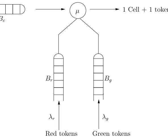
The Leaky Bucket (LB) [17] is an access control mechanism in the ATM network. This control is performed using tokens. These tokens are given to each cell when it enters the network. This mechanism may be im-plemented in several ways. We focus on the one called the Virtual Leaky Bucket (VLB) [18]. In this kind of LB, three buffers are needed. The first one welcomes the user’s cells, and the others are respectively used for green and red tokens. When a cell arrives in the first buffer Bc, if that one is not full, it is kept there waiting to be served. A service to a cell consists in giving it a green token coming from the buffer Bg. This token represents its permission to access into the network. Otherwise, if Bc is full, the cell may be lost (rejected), even if the network has sufficient resources to accept it, without altering the quality of service. In order to avoid this situation, red tokens are generated by the bufferBr. A threshold S is fixed. If Bg is empty while there are less thanS cells in Bc, those cells should wait for new green tokens to be generated, before they enter the network. On the contrary, if there are more thanS cells inBc whenBg is empty, they should be able to access the network with red tokens if, of course,Br is not empty. This mechanism is described by figure 4.1.
λ
cλ
rλ
gµ
1 Cell + 1 token
Cells
Red tokens
Green tokens
B
rB
gB
cFig. 4.1.The Virtual Leaky Bucket
The ATM mechanism is modeled by a SAN composed with three automata A(1), A(2) and A(3). These
automata represent respectively the content of buffers Bc, Bg and Br. Each automatonA(k) is supposed to
havesnk states, k= 1,2,3. These states are numbered from 0 tonk−1. The threshold of bufferBc is set to
S. The events that occur in the system are as follows:
• Local events
— arrival of a cell with rate λc, a local event toA(1)
— arrival of a green token with rate λg, a local event toA(2)
— arrival of a red token with rate λr, a local event toA(3).
• Synchronizing events
— s1: departure of a cell with a green token (rateµ), acting on bothA(1) andA(2)
— s2: departure of a cell with a red token (rateµ), acting on bothA(1) andA(3).
Figure 4.2 shows the behaviour of each automaton for the case wheren1= 4,n2=n3= 3 and S= 1.
The transitions inA(1) are either cells arrivals (with rateλc) or cells departures (service). A departure is
A
(1)A
(2)A
(3)0
1
2
3
(
s
1, µ,
1)
×
(
s
2, µ,
1)
(
s
1, µ,
1)
×
(
s
2, µ,
1)
λ
cλ
cλ
c(
s
1, µ,
1)
0
1
2
(
s
1, µ,
1)
(
s
1, µ,
1)
(
s
2, µ,
1)
λ
gλ
g0
1
2
(
s
2, µ,
1)
(
s
2, µ,
1)
λ
rλ
rFig. 4.2.The automata transitions diagram of the SAN associated to the Virtual Leaky Bucket
thanS and red if not). The service rate is alwaysµ and the occurrence probability (routing probability) is 1, only one choice being possible. The transitions inA(2) and A(3) are arrivals (with ratesλg or λr) of green or
red tokens or their departures. A token departure means that a cell has been served, therefore synchronization eventss1 ands2 stand. These transitions have rateµand also an occurrence probability equals to 1. The fact
that a red token is usable only whenBg is empty is modeled by the loop around state 0 of automatonA(2).
The SAN modeling the VLB is determined by the descriptorQand the initial distribution Π(0) as follows. Let be, fork= 1,2,3,
Q(k)the infinitesimal generator associated to automatonA(k),
E1(k)the positive event matrix of events1 over automatonA(k), and
E2(k)the positive event matrix of events2 over automatonA(k).
Thedescriptoris given by
Q=Q(1)⊕Q(2)⊕Q(3)+E1(1)⊗E (2) 1 ⊗E
(3) 1 +E
(1) 2 ⊗E
(2) 2 ⊗E
(3) 2 .
If Π(k)(0),k= 1, 2, 3,denotes the initial distribution of thekthautomatonA(k), we have Π(k)
1 (0) = 1 and for
i≥2, Π(ik)(0) = 0. The global initial distribution (of the SAN) is Π(0) such that Π(0) =⊗3
4.2. Performance analysis. In order to compute the vector Π(t) for our SAN model, we considern1=
256,n2= 128 andn3= 32. This situation means that buffersBc,BgandBrhave a limited capacity of 255, 127
et 31 respectively. The thresholdSis fixed to 200. Thus, the descriptorQhas an orderM = 220andthe system has 1.048.576 states. It is important to note that only the matricesQ(k) and E(k)
i , k= 1,2,3 andi= 1,2,
are stored by using a compact storage scheme. The rates values are such that λb =λc =λ= 0.5 andµ= 1. For evaluating the performance of our global algorithm, we execute it on a cray t3e, a distributed memory parallel machine. It possesses up to 256 processing elements, each running at 300 MHZ. The computations of the program (written in Fortran) are done in numerical arithmetic double precision.
We first focus on the CPU time of our algorithm as function of the mission time t and the number of processorsP. We considert= 10i,i= 0, . . . ,5 andP = 32,64,128. Next, we compute the speedupSP and the
efficiencyEP as function ofP. For the SU method, the value ofεis fixed to 10−10 (cf. relation (2.7)).
Table 4.1
CPU time (s) for computingΠ(t)as function oftandP
t 1 10 102 103 104 105
P=32 61.72 222.17 1745.45 14599.34 137696.21 (e) 1350907.9 (e)
P=64 30.55 137.76 912 7628.15 71945 (e) 705842.6 (e)
P=128 1.6 7.96 48.16 427.93 3791.89 37201.16
Table 4.1 includes the CPU time values for computing Π(t) as function of t and P. In this table, the notation (e) means that corresponding CPU time values are estimated taking advantage of the SU method for estimating a priori the time complexity. A lecture of this table shows that even whent= 105, the vector Π(t)
can be evaluated with 128 processors in about 10 CPU hours. This table also shows the feasibility limits of some problems as function of the state space size M, mission time t, and number of processorsP. Speedup
Table 4.2
Speedup and efficiency as function ofP
P 32 64 128
SP 29 54 100
EP 0.90 0.84 0.78
and efficiency, as function ofP, are given in Table 4.2. The values of SP increases with P; the CPU times is then inversely proportional toP. Table 4.2 shows that the value of EP remains in average greater than 80%, meaning a good use of processors and a low communication time.
It is important to note that the given numerical results depend on the SAN model. The speedup SP
decreases when N increases [19]. It is then possible to aggregate some automata [20] in order to obtain the same value of N. The mean number α of non-zero terms in rows or columns of matrices used in the tensor sums and products increases without modifying significantly the efficiencyEP. If we consider complex SANs for whichNis large (N increases), it is difficult to predict the expected speedup starting from the given application. More complex applications constitute the goal of our future work.
REFERENCES
[1] B. Plateau,On the Stochastic Structure of Parallelism and Synchronisation Models for Distributed Algorithms,Performance Evaluation, 13(5):142–154, 1985.
[2] W. J. Stewart, K. Atif, and B. Plateau,The numerical solution of stochastic automata networks, European Journal of Operation Research, 86:503–525, 1995.
[3] B. Plateau, On the Stochastic Structure of Parallelism and Synchronisation Model for Distributed Systems, ACM SIG-METRICS conference On Measurement and Modeling of Computer Systems, pages 147–153, May 1985.
[4] B. Plateau and K. Atif, Stochastic Automata Networks for Modelling Parallel Systems, IEEE Transactions On Software Engineering, 17(10):1093–1108, 1991.
[5] M. S. Bebbington, Parallel implementation of an aggregation/disaggregation method for evaluating quasi-stationary be-haviour in continuous-time Markov chains, Parallel Computing, 23:1545–1559, 1997.
[6] J. K. Muppala M. Malhotra, K. S. Trivedi, Stiffness-tolerant methods for transient analysis of stiff Markov chains, Microelectronic Reliability, 34(11):1825–1841, 1994.
[7] K. S. Trivedi and A. L. Riebman,Numerical Transient Analysis of Markov Models, Computer and Operations Research, 15(1):19–36, 1988.
[8] H. Abdallah and R. Marie,The Uniformized Power Method for Transient Solutions of Markov Processes,Computers and Operations Research, 20(5):515–526, April 1993.
[9] C. Lindemann, M. Malhotra and K. S. Trivedi, Numerical Methods for Reliability Evaluation of Markov Closed Fault-Tolerant Systems, IEEE Transactions on Reliability, 44(4):694–704, 1995.
[10] H. Abdallah and M. Hamza, Sensitivity analysis of instantaneous transient measures of highly reliable systems 11th
European Simulation Symposium (ESS’99), Erlangen-Nuremberg, Germany, october 26-28, pages 652–656, 1999. [11] C. Tadonki and B. Philippe, Parallel Multiplication of a Vector by a Kronecker Product of Matrices (part I), Parallel and
Distributed Computing Practices, 2(4):413–427, December 1999.
[12] H. Abdallah and M. Hamza, Sensitivity analysis of the expected accumulated reward using uniformization and IRK3 methods, Second Conference on Numerical Analysis and Applications (NAA’2000), Rousse, Bulgaria, June 11-15, 2000. [13] M. Davio, Kronecker Products and Shuffle Algebra IEEE Transactions on Computers, 30:116–125, 1981.
[14] D. P. Bertsekas and J. N. Tsitsiklis, Parallel and Distributed Computing. Prentice-Hall, Englewood Cliffs, N. J., 1988. [15] S. M. Mller A. Bingert, A. Formella and W. J. Paul, Isolating the Reasons for the Performance of Parallel Machines
on Numerical Programs, In International Workshop on Automatic Distributed Memory Parallelization, Automatic Data Distribution and Automatic Parallel Performace Prediction, pages 34–64, Austin, Texas, USA, 1993.
[16] B. Weiss ATM. Hermes, Paris, 1995.
[17] I. Cidon and I. S. Gopal, An approach to Integrated High-Speed Private Network, International Journal on Digital and Analogical Systems, 1:77–86, 1988.
[18] M. Hirano and N. Watanabe,Characteristics of a cell multiplexer for bursty ATM traffic, IEEE ICC’89, pages 1321–1325, 1989.
[19] C. Tadonki and B. Philippe, Parallel Multiplication of a Vector by a Kronecker Product of Matrices (part II),Parallel and Distributed Computing Practices, 3(3), September 2000.
[20] O. Gusak, T. Dayar, and J. M. Fourneau, Lumpable continuous-time stochastic automata networks, International Conference on Mathematical Modeling and Scientific Computing, Middle East Technical University and Selcuk University, Ankara and Konya, Turkey, April 2001.