doi: 10.1098/rspa.2003.1163
, 3079-3098
459
2003
Proc. R. Soc. Lond. A
Alexander M. Leshansky, Olga M. Lavrenteva and Avinoam Nir
The weakly inertial settling of particles in a viscous fluid
Email alerting service
corner of the article or click Receive free email alerts when new articles cite this article - sign up in the box at the top right-handherehttp://rspa.royalsocietypublishing.org/subscriptions go to:
Proc. R. Soc. Lond. A
To subscribe to
10.1098/rspa.2003.1163
The weakly inertial settling of particles
in a viscous fluid
B y A l e x a n d e r M. L e s h a n s k y1, O l g a M. L a v r e n t e v a2
a n d A v i n o a m N i r2
1Division of Chemistry and Chemical Engineering,
California Institute of Technology, Pasadena, CA 91125, USA
2Department of Chemical Engineering,
Technion—Israel Institute of Technology, Haifa 32000, Israel
Received 15 January 2003; accepted 2 April 2003; published online 1 October 2003
In this paper we investigate the influence of fluid inertia on the settling of a finite assemblage of solid spherical particles in a constant gravity field at small Reynolds number,Re. We show that the first effect of fluid inertia on particle velocities scales as Re, for times much larger than the viscous-relaxation time. In this case the Eulerian acceleration terms associated with the unsteadiness of the stresslet in the far velocity field and the entire local fluid inertia (acceleration and advective terms) contribute at O(Re). As a particular example, Oseen velocities are calculated of two spheres falling along the line of their centres. The inertia-induced relative motion between the particles is in excellent agreement with previous experimental results.
Keywords: sedimentation; inertia; hydrodynamic interaction
1. Introduction
Many classical and novel engineering processes involving multiphase flow require advanced theoretical models that are capable of describing correctly the collective phenomena that govern the motion of assemblies of small particles in a viscous fluid. Perhaps the most extensively studied case is the classical problem of passive sedi-mentation of particles in a constant gravity field. Many theoretical models that were developed to simulate the dynamics of many interacting particles in a viscous fluid have invariably adopted the quasi-steady zero-Reynolds-number (Re= 0) approach by completely ignoring the transient and nonlinear inertia effects (Brady & Bossis 1988; Hassonjeeet al. 1988; Mo & Sangani 1994; Sierou & Brady 2001). Due to this approach, at a given time, the velocities of all particles are determined by force and torque balances for an instantaneous geometric configuration of the assemblage and the motion of each particle is controlled by its translation velocity at the current time. Although, under the viscous limit, Re = 0, the equations of fluid motion are linear (using the Stokes or creeping-flow model), long-range hydrodynamic interac-tions between particles mediated by the fluid are highly nonlinear and the dynamics of even several particles can be quite complex: unstable separating configurations (Hocking 1964), periodic or quasi-periodic trajectories (Hocking 1964; Caflischet al.
1988; Golubitsky et al. 1991; Snook et al. 1997) and chaotic solutions (J´anosi et al. 1997) were found for three sedimenting particles, while Durlofsky et al. (1987) constructed a periodic solution for configurations of four and eight particles.
It is widely believed that the creeping-flow model gives reasonably accurate results up to Re ≈ 1, while the validity of neglecting the inertia of both the particles and the fluid has not been rigorously justified. For example, the widely used so-called Stokeslet model, where the moving particles are approximated by point-like objects, is only asymptotically valid whenRe s/a→0 and a/s→0, wherea is the radius of the spherical particles andsis a typical distance between spheres.
We are aware of only a few works that examine the validity of the quasi-steady approach in multi-particle systems. Oseen (1927) (see Happel & Brenner 1965, pp. 281–283) used a reflection technique for two spheres in a creeping motion while using single-sphere Oseen velocity fields instead of Stokes fields to approx-imate weakly inertial particle interaction. As pointed out by Happel & Brenner (1965), the Oseen equations do not correctly approximate the boundary conditions on the spheres’ surfaces and thus Oseen’s results for the two-sphere problem must be regarded with suspicion. Jayaweeraet al. (1964) experimentally observed expansion of the regular polygon configuration of the settling spheres during their settling and the damping of the oscillations about their mean relative positions, which cannot be explained in the framework of the creeping-flow model.
Leichtberg et al. (1976) reported a study of the coaxial sedimentation of three identical spheres. By using the expression for the Basset force of a single sphere, they found that the deviation in the particle position from that predicted by zero-Reynolds-number theory grows with time as t1/2, due to integrated effects of the unsteady Basset force. In fact, they could not formulate the correct Basset force for each sphere in the presence of other particles and had to use the Basset force for a single sphere in the dynamic-force equation. Feng & Joseph (1995) considered the unsteadiness due to hydrodynamic inter-particle interaction or due to particle interaction with the wall. They assumed, using scaling arguments, that the transient inertia terms in the equations of motion would dominate over the quadratic inertia terms at small Reynolds numbers. Using numerical simulations of the transient Stokes equations, they showed that a small amount of fluid inertia can significantly modify the quasi-steady trajectories of particle motion in the long-time limit. Although they mention that if the entire fluid inertia is considered, the solution may look quite different from that which they have obtained taking into account the unsteady fluid inertia only, the question of when the nonlinear convective inertia terms should be retained in the governing equations remained open.
Recently, Leshanskyet al. (2003) considered the dynamics of a particle assemblage in an arbitrary slowly varying uniform flow at lowRe. It was shown that when the Stokeslet in the disturbance far velocity field is time dependent, there is a Basset history-type contribution to the particles’ velocities, which scales as√Re, and is the same for all particles in the assemblage. Moreover, this theory suggested that when there is a constant Stokeslet in the far velocity field, e.g. sedimentation in a fluid that is quiescent at infinity, the above Basset contribution vanishes and the first effect of the fluid inertia on the particles’ velocity reduces toO(Re).
Re is obtained. Consequently, we revisit the classical problem of coaxial settling of two spheres, calculating the Oseen velocity for each separation distance.
2. Statement of the problem
Consider a gravitational settling of a finite assemblage ofnrigid particles of massmi and density ρsi in a viscous Newtonian fluid quiescent at infinity, with density and viscosity equal to ρ and µ, respectively. Let x = (x1, x2, x3) be a radius vector to a point in the laboratory coordinate system with some chosen origin. If we suppose that the particles are spherical, then the domain occupied by the continuous phase may be represented by D(t) = {x ∈ R3 : |x−Z
i(t)| > ai, i= 1,2, . . . , n}, where Zi(t) denotes a radius vector to the centre of theith particle andai stands for the particle radius. Thus the velocity field v(x, t) = (v1, v2, v3) and the pressurep(x, t) are described by the following equations and boundary conditions,
∂v
∂t +v· ∇v=−ρ
−1∇p+ν∆v+g, x∈ D(t), (2.1)
∇ ·v= 0, x∈ D(t), (2.2)
v=ui(x, t), x∈Γi(t), (2.3)
and
v→0, p→p∞(x) as|x−Y(t)| → ∞, (2.4)
whereΓi(t) denotes the surface of the ith particle, ui(x, t) is the velocity at points on the surface of the ith particle, and Y(t) stands for the position vector of some reference point that lies inside the swarm. Since the particles are rigid,
ui=Ui(t) +Ωi(t)×ri,
whereUi andΩiare the linear and angular velocities of motion andri(t) =x−Zi(t) is the radius vector with its origin at the centre ofith particle. The dynamic force and torque balance (about the centre ofith particle) at any moment are given by
mi dUi
dt =
Γi
σ·nds+mig, (2.5)
Ii dΩi
dt =
Γi
ri×(σ·n) ds, (2.6)
whereσ=−pI+µ(∇v+ (∇v)T) is the stress tensor andm
i andIi denote the mass and moment of inertia of the particle, respectively. The problem is completed by the kinematic condition
Ui = ˙Zi(t), i= 1,2, . . . , n, (2.7)
where a dot denotes the time derivative and, by the initial conditions,
Zi(0) =Zi0, Ui(0) =Ωi(0) =0, i= 1,2, . . . , n, (2.8)
v(x,0) =0, x∈ D(0). (2.9)
We pose the problem formulation in a co-moving coordinate frame with its origin at the reference pointY(t) lying instantaneously inside the swarm, i.e.
x=x−
t
0
while we assumea priorithat the velocity of the reference point,U(t), can be chosen to be aligned with the direction of the gravitational acceleration, g, so that the condition max{|Y −Zi|} L, where L denotes the assemblage spatial dimension, is fulfilled on durations of interest.
Since we want to focus on thedisturbances of the velocity and pressure fields that vanish at infinity, we introduce the pressure disturbance
p=p−ρg·x. (2.11)
The following scaling is chosen: the typical radius of a particle, a, for length; the magnitude of a settling velocity of an isolated particle, uo = a2g(λ−1)/ν, where g=|g|and λ=ρs/ρ is a typical density ratio, for velocity; Stokes time,tS=a/uo, for time; andµuo/afor pressure. Assume further that the Stokes time unit is much larger than that of the viscous-relaxation time based on the assemblage dimension, tS tν, where tν = L2/ν, which means that a quasi-steady velocity field in the vicinity of the assemblage is immediately established.
In dimensionless form, after omitting the primes, the velocity and pressure fields should satisfy
Re
∂v
∂t + (v−U)· ∇v
=−∇p+ ∆v, x∈ D(t), (2.12)
∇ ·v= 0, x∈ D(t), (2.13)
v=ui, x∈Γi(t), (2.14)
and
v, p→0 as |x| → ∞, (2.15)
where Re = uoa/ν is the Reynolds number and U is the velocity of the reference point. Conditions (2.7)–(2.9) in dimensionless form remain unchanged, while the dynamic force and torque balances (2.5) and (2.6) become
˜
miReUi˙ =
Γi
σ·nds+e˜vi
λi−1 λ−1
, (2.16)
˜
IiReΩ˙i =Ri
Γi
n×(σ·n) ds, (2.17)
where e= g/g, ˜mi is the mass of the particle non-dimensionalized by the product ρa3, ˜Ii is the moment of inertia of the particle scaled by the productρa5, λi=ρsi/ρ is a density ratio of theith particle, Ri = ai/a stands for the dimensionless radius and ˜vi= ˜miλ−i 1 is a dimensionless volume of the particle. In (2.16), we made use of
the equality
Γi
(e·x)nds=e˜vi.
3. Construction of the solution for small Re (a) Basic assumptions and zero-order approximation
solution of (2.12)–(2.17) under the assumption ofRe= 0. The position of each par-ticle, Zi, varies with time since, although the velocity field is found as a solution of non-evolutionary problems, it depend on time parametrically via the evolution of the problem domain. It is obvious that the quasi-steady solution cannot satisfy the initial conditions (2.8), (2.9) and a time-scaleO(tν) must exist, representing the initial period of rapid acceleration from rest. Rescaling of the dimensionless time as t∗ =Re−1tshows that, in the initial period, all three terms in (2.16) are of the same order of magnitude, the unsteady term in (2.12) is O(1), while the nonlinear con-vective term still can be neglected due to the smallness of the velocity disturbance. Therefore, during this initial period, the unsteady inertial, virtual-mass and Basset forces would be comparable. Nevertheless, the initial transient phase is short-lived (Kim & Karrila 1991) and, in the case of an isolated particle, it has been found that the temporal decay to the steady-state is faster than thet−1/2 behaviour (Lovalenti & Brady 1993).
In what follows we shall focus on the long-time behaviour of the assemblage. More specifically, we are interested in the leading-order inertial corrections to the quasi-steady particles’ velocities
ui=u0i +f(Re)u1i +o(f(Re)), f(Re)1.
ForRe= 0, the problem formulated in (2.12)–(2.17) is a Stokes problem. Using the boundary integral representation of the velocity field,v0, corresponding to Re= 0, and eliminating the double-layer integral (Pozrikidis 1992), we arrive at
v0 =− 1
8π
S
(σ0(y)·n)·G(x−y) ds(y), (3.1)
where S=∪iΓi is a multiply connected solid surface and G is the Oseen–Burgers tensor orStokeslet with components
Gij(x) = δij r +
xixj r3 ,
wherer=|x|. Far from the swarm,r |y|, the leading term of the disturbance field can be found by using the multipole expansion of the integral representation for the velocity and pressure (Kim & Karrila 1991),
v0=−F
0·G(x)
8π +
S0· ∇G(x)
8π +O(r
−3), (3.2)
p0=−F
0·P(x)
8π +
S0· ∇P(x)
8π +O(r
−4), (3.3)
whereP is the pressure vector with components Pi= 2xi/r3 and
Fj0=
S
(σ0·n)jds, (3.4)
Sjk0 = 1
2
S
[(σ0·n)jyk+ (σ0·n)kyj] ds− 13δjk
S
(σ0·n)·yds. (3.5)
(the antisymmetric part of the force dipole, a rotlet, is absent, since particles are free to rotate). Under the assumption of creeping flow, the net drag force exerted on falling particles by the fluid is independent of the configuration and is balanced entirely by buoyancy. If particles are not too heavy ( ˜miRe1), the particle inertia terms on the left-hand side of (2.16) can be neglected to a first approximation and it follows that
F0=
i
Γi
σ0(y)·nds=−e
i ˜ vi
λi−1 λ−1
=F0e. (3.6)
Note thatS0 is generally a time-dependent tensor.
(b) General asymptotic theory
Let the vector function
H={v(x, t), p(x, t),U1(t),U2(t), . . . ,Un(t),Ω1(t), . . . ,Ωn(t),Z1(t), . . . ,Zn(t)} be a solution of problem (2.12)–(2.17). Its projectionF ={v(x, t), p(x, t)}will also be considered. For 0< Re1, let the above solution be presented in the form
H=H0+ReH1+O(Re2),
where the superscript ‘0’ corresponds to the above-mentioned quasi-steady solution withRe= 0. It is clear that aregularexpansion of the solution in integer powers ofRe breaks down, since the Eulerian acceleration terms,∂v0/∂t, and the advective inertia terms,U· ∇v0, decay asr−2 far from the assemblage and thus the first correction of the velocity field,v1, does not possess solutions that vanish at infinity. Following a well-established procedure (van Dyke 1975), we construct inner and outer expansions ofH and F, respectively. The inner expansion, Hin, satisfies (2.12)–(2.17), except the condition (2.15) at infinity, and the outer expansion, which concerns only the projection ofH,
Fout={V(ζ, t), P(ζ, t)}, ζ=εx∈R3\ {0}, t >0,
where 0< ε(Re)1 is some small parameter to be chosen later, should satisfy (2.12) and (2.13) and vanish at infinity,
lim
|ζ|→∞Fout=0. (3.7)
The projection of the inner expansion,Fin, and the above outer expansion match asymptotically,
Fout(|ζ| →0)Fin(|x| → ∞). (3.8) We assume that the inner and the outer expansion may be represented, respectively, by
Fout=
∞
n=1
ωn(Re)·Fnout, Hin=
∞
n=1
χn(Re)·Hnin, (3.9)
whereω and χ are diagonal matrices of the expansion coefficients, with their com-ponents satisfying (no summation)
lim Re→0
ωiin+1 ωn
ii
= 0, lim
Re→0
χn+1ii χn
ii
The first term of the inner expansion is a solution of a quasi-steady problem corre-sponding toRe = 0 and, therefore, χ0 =I. This procedure suffices when the inner and outer regions overlap and conditions (3.7) and (3.8) can be satisfied. As shown below, generally this is not true and the standard two-region procedure described here must be extended to include a three-region expansion: an innerviscous region, an intermediatetransient viscous region and a far outer Oseen region.
(c) The first and the second term of the outer expansion
Let Fout = {V(ξ, t), P(ξ, t)} = {v(ξ/ε, t),p(ξ/ε, t)}, where 0 < ε(Re) 1 is some small parameter to be determined. In terms of the outer spatial variable, equa-tion (2.12) becomes
Re
∂V
∂t +ε(V −U)· ∇ξV
=−ε∇ξP +ε2∆ξV. (3.10)
The form of (3.10) suggests thatFoutpossesses the asymptotic expansions (3.9) with
ω0=ω0(ε)
1 0 0 ε
, ω1 =ω1(ε)
1 0 0 ε
, (3.11)
where the functions Vn and Pn should vanish as |ξ| → ∞. It follows that the appropriate choice of the expansion parameter is ε=√Re. Under this choice, the leading term of the outer expansion,F0out, in (3.9) is a fundamental solution of the steady Stokes equation
−∇ξP0+ ∆ξV0= 0, (3.12)
which matches exactly the Stokeslet term in the far-field expansion of the quasi-steady solution (3.2), (3.3),†
ω0(ε)V0(ξ, t) =−εF
0·G(ξ)
8π , εω
0(ε)P0(ξ, t) =−ε2F0·P(ξ)
8π . (3.13)
It follows from (3.13) thatω0=ε.
The second term of the outer expansion, F1out, satisfies the non-homogeneous transient Stokes equation,
∂V1
∂t +∇ξP 1−∆
ξV1=U· ∇ξV0, (3.14)
and matches the stresslet term in the outer limit of the quasi-steady zeroResolution in (3.2), (3.3) in the vicinity ofξ=0,
ω1(ε)V1(ξ, t)ε2S
0(t)· ∇G(ξ)
8π , εω
1(ε)P1(ξ, t)ε3S0(t)· ∇P(ξ)
8π . (3.15)
It readily follows from these matching conditions thatω1=ε2=Re. Note that the terms on the right-hand side of (3.14),U · ∇ξV0, are ofO(|ξ|−2) and thus we are not able to find solutions that vanish at infinity and satisfy condition (3.7). This
brings us to the conclusion that there must be a far outer region at r ∼ Re−1, i.e. theOseen region, where the inertia advective terms are balanced by the viscous terms in (3.10), and that the region discussed so far is anintermediate outer region. The Oseen solution in the far outer region should match the leading term of the
intermediate outer expansion and also provide an appropriate outer limit for the second term of the intermediate outer expansion,V1, governed by (3.14). Thus the present problem possesses a three-region structure, while both the far Oseen region and the intermediate outer region would contribute to the inner solution atO(Re).
Let{V(ζ),P(ζ)}correspond to an outer Oseen solution of (2.12), whereζ=Rex. Since the Oseen solution should match the Stokeslet term in the intermediate outer region at the first approximation,
V(ζ, t)V0(ε−1ζ, t) =−ReF
0·G(ζ)
8π as|ζ| →0, (3.16)
we assume that the Oseen velocity and pressure fields possess the following asymp-totes: V ReV0, P Re2P0. It follows from (2.12) that the leading term of the Oseen outer expansion is governed by
−U· ∇ζV0 =−∇ζP0+ ∆ζV0, (3.17)
while we require that V0 and P0 should vanish at |ζ| → ∞. The solution of (3.17) driven by a point-force singularity at the origin (equation (3.16)) is given in the appendix. Asymptotic expansion of the outer Oseen solution at the vicinity ofζ=0 results in the proper outer limit of the velocity field in the intermediate region,
V(ξ, t) −εF
0·G(ξ)
8π +ε
2(F0·e)A(ρ−1ξ)
8π as|ξ| → ∞, (3.18)
whereρ=εr =|ξ| and A:S2 →R3 is a vector-valued function on the unit sphere
S2 inR3, with components given by
Ai(ρ−1ξ) = 12U
ei+ 1
ρ(ejξj)ei− 1 2ρ
1− 1 ρ2(ejξj)
2
ξi
. (3.19)
Using (3.17) and (A 2), we find that the pressure in the Oseen region is not per-turbed, and hence
P0=−F0cosθ 4π2 =−
F0·P(ζ)
8π =−ε
2F0·P(ξ) 8π ,
i.e. it exactly matches the Stokesian pressure term in the intermediate region. Having at hand the proper behaviour of V(ξ, t) as |ξ| → ∞ at ε2, we can now proceed with the construction of the solution of (3.14) in the intermediate outer region. Note that
Vp1= F
0A(ρ−1ξ)
8π
transient Stokes equation corresponding to (3.14), driven by a varying symmetric force dipole singularity at ξ = 0 due to (3.15) and vanishing at infinity. Let us denote the solution of the latter problem by{V1
h, Ph1}, while
∂V1 h
∂t +∇ξP 1
h −∆ξVh1 = 0, ξ∈R3\ {0}, t >0, (3.20)
and
Vh1 S
0(t)· ∇G(ξ)
8π , |ξ| →0, (3.21)
Ph1 S
0(t)· ∇P(ξ)
8π , |ξ| →0, (3.22)
{Vh1, Ph1} →0, |ξ| → ∞. (3.23) Vh1 andPh1 can be found by differentiating the fundamental solution of the transient Stokes equation (Kim & Karrila 1991) as
ˆ
Vh1(ξ, s) =
ˆ
S0· ∇
ξGˆ(ξ;s)
8π , Pˆ
1
h(ξ, s) = ˆ
S0· ∇
ξP(ξ)
8π ,
where ˆG(ξ;s) denotes a transient Oseen tensor with components
ˆ
Gij(ξ;s) = 4
ρ3s2[1−(1 +ρ √
s)e−ρ√s]ξiξj ρ2
+ 2
ρ3s2[(1 +ρ √
s+ρ2s)e−ρ√s−1]
δij− ξiξj
ρ2
(3.24)
and Pi(ξ) = 2ξi/ρ3. Here, symbols with hats refer to the Laplace images of the corresponding variables. Expanding a two-term outer solution near ρ = 0, then rewriting it in terms of the inner spatial variables up to O(ε2) and transforming back to the time domain, t, the outer (inner) limit of the inner (outer) solution is found as
Vi= 1 8π(−F
0
j · Gij(x) +S 0
jk· Gij,k(x))
+ ε 2
8π( ˙S 0
jk· Bijk(r− 1
x) + (Fj0·ej)Ai(r−1x)) +o(ε2), (3.25)
P = 1 8π(−F
0
j · Pj(x) +S 0
jk· Pj,k(x)) +o(ε 2
), (3.26)
whereB(r−1x) is the third-rank tensor on the unit sphereS2inR3with components
Bijk = 1 2
xkδij r +
xixjxk r3
, (3.27)
and it is assumed thatS0(−∞) =0, which indicates that we neglect the influence of the short-lived initial transient on the long-time behaviour of the assemblage. The form of (3.25) and (3.11) suggests that the second term of the inner expansion should be of the order ofε2 =Re andχ1 =ε2I, or simply
The term ofO(ε2) in (3.25) proportional to ˙S0is associated with an unsteadiness of the flow due to the inter-particle interactions. TheO(ε2) term in (3.25) reduces to the classical Oseen term when the quasi-steady solution is time independent, e.g. the settling of two identical spheres or regular horizontal polygons of identical spheres.
(d) The second term of the inner expansion
The second term in the inner expansion ofHshould satisfy the non-homogeneous Stokes equation and the following conditions at the particle boundaries and far from the assemblage,
−∇p1+ ∆v1 =W0(x, t), x∈ D, (3.28)
∇ ·v1 = 0, x∈ D, (3.29)
v1 =u1i −Zi1· ∇v0, x∈Γi0, (3.30)
and
v1→(8π)−1((F0·e)A+ ˙S0·B), p1→0 as|x| → ∞, (3.31)
where
W0(x, t) = ∂v0 ∂t + (v
0−U)· ∇v0,
Bis given by (3.27) andAis defined in (3.19). It is readily seen that there are three contributions to the solution at this order:
(i) the advection of momentum from the far Oseen region corresponding to the term proportional to the Stokeslet strength in (3.31);
(ii) the unsteady inertia in the intermediate outer region corresponding to the term proportional to the rate of change of the stresslet in (3.31);
(iii) the local inertia of the fluid in the inner region, corresponding to the right-hand side of (3.28).
Note that the entire local fluid inertia withinW0 contributes at the leading order. The boundary conditions (3.30) are applied at the undisturbed particles’ surfaces, Γi0(t), corresponding to their quasi-steady positions, Zi(t) = Zi0(t). The dynamic force and torque balances (2.16), (2.17) at O(ε2) calculated on the unperturbed particles’ surfaces give
˜ miU˙i0=
Γ0
i
[σ1·n+K1] ds, (3.32)
˜
IiΩ˙i0=Ri
Γ0
i
[n×(σ1·n+K1) +K2] ds, (3.33)
where the second-rank tensors are given by
K1(Z1;σ0,∇σ0) =Zi1·
σ0
Ri ·
(I−nn) +∇σ0·n
,
The terms proportional toZ1 appear in (3.32) and (3.33) due to the disturbance of the boundary,Γi. Taking advantage of the quasi-stationary nature of the perturbed problem, we solve the problem formulated in (3.28)–(3.33) for a disturbed boundary, Γi. Thus, on each time-step,Γi is approximated in accordance with their calculated velocities by a finite-difference method and the problem formulated in (3.28)–(3.33) is resolved for the newly found particle positions, while the terms proportional to Z1 in (3.30) and in (3.32) and (3.33) are set to zero. In some special cases, e.g. set-tling of regular horizontal polygons ofN identical spheres or coaxial sedimentation of two spheres, the trajectories are known due to symmetry (up to time parametriza-tion), and therefore it is enough to calculate disturbed particle velocities along these prescribed trajectories.
We may seek the solution of (3.28)–(3.33) in the form
F1
=F10+F11+F12,
whereF11 ={v1
1,0}={(F0A+ ˙S0·B)/8π,0}and F12={v12, p12}correspond to the solutions of the non-homogeneous Stokes equations (3.28), (3.29) with the right-hand sideW0= (W−∆v11) given by volume potentials (Ladyzhenskaya 1969)
v21(x, t) =− 1
8π
R3
W0
∗(y, t)·G(x−y) dv(y), (3.34)
σ21(x, t) = 1
8π
R3
W0
∗(y, t)·T(x−y) dv(y), (3.35)
where W0
∗ is a smooth regular continuation of W0 onto R3 and T(x) is a stress
tensor with components
Tijk(x) =−6 xixjxk
r5 . ThusF10={v1
0, p10}is a solution of homogeneous Stokes equations and should satisfy the following boundary conditions:
v10 →0 as |x| → ∞, (3.36)
v10 =u1i −v11−v12, x∈Γi. (3.37)
The force and the torque balance (3.32), (3.33) would become
˜ miU˙i0 =
Γi
σ10·nds+F1i1 +F2i1, (3.38)
˜
IiΩ˙0i =Ri
Γi
n×(σ10·n) ds+T1i1 +T2i1, (3.39)
where {F11,T11}i and {F21,T21}i correspond to a force and a torque exerted by the fluid on the ith particle by F11 and by F12, respectively. Thus the above solution decomposition leads us to a homogeneous Stokes problem with a prescribed velocity and pressure distribution on the surface of the particles.
4. Numerical results and discussion
0 5 10 15 20 separation
−0.06 −0.05 −0.04 −0.03 −0.02
U
1 1,
U
[image:13.612.191.409.72.210.2]1 2
Figure 1. The Oseen velocity of equal-size spheres falling along the line of their centres. The dashed line corresponds to the velocity of the trailing particle; the solid line corresponds to that of the leading particle.
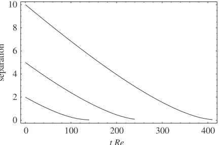
0 100 200 300 400
t Re 0
2 4 6 8 10
separation
Figure 2. Inter-particle separation distance between two coaxial equal-size spheres as a function of stretched dimensionless time,tRe, for different initial separations.
equal Stokes velocities and, hence, the basic solution in a reference frame fixed with the particles is independent of time, the intermediate outer region atr ∼aRe−1/2 vanishes and the correction is due to the Oseen outer region contribution and the local inertia in the vicinity of the spheres. The velocity and stress distribution, v1 2 andσ1
2 in (3.34) and (3.35), respectively, are calculated in cylindrical coordinates on the surface of the particles, while the appropriate expressions for the axisymmetric
kernelsGandT can be written in terms of complete elliptic integrals of the first and second kind (Pozrikidis 1992). Taking advantage of the axial symmetry, we find an analytic solution to the Stokes problem forv1
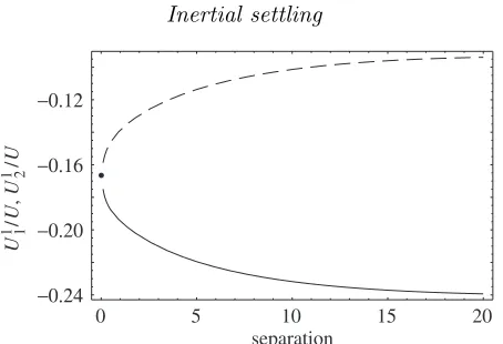
[image:13.612.194.412.261.404.2]0 5 10 15 20 separation
−0.24 −0.20 −0.16 −0.12
U
1 1/
U
,
U
1 2 /
U
[image:14.612.187.414.56.211.2]•
Figure 3. The rescaled Oseen velocity of equal-size spheres falling along the line of their centres.
O(1). To illustrate this, we integrate the equation of the particles’ relative motion,
˙
Z(t) =U1−U2 =Ur(Z(t)),
whereZ(t) =Z1(t)−Z2(t) is the separation distance between the particles’ centres, and plot in figure 2 the separation distance between their surfaces,Z−2, as a function of a rescaled dimensionless time,tRe. These results suggest, for instance, that even for small enough Re 0.1, around 1000 Stokes times are required to observe the decrease in the inter-particle separation from 5 to 2.5.
This behaviour is in qualitative agreement with Oseen’s approximate solution (Oseen 1927 (as in Happel & Brenner 1965, pp. 281–283)), who used a reflection method for two spheres in a creeping motion while substituting Oseen velocity fields instead of Stokes fields to approximate the weakly inertial particle interaction. For small values of the product RepZ, the velocity of the leading particle decreases by subtracting 38Rep from its Stokes value, while the velocity of the trailing particle is unaltered by the fluid inertia. Here,Rep=U0a/ν is the Reynolds number based on thepairwisesettling velocity of the particle in the case of creeping-flow equation, and, therefore, Rep varies with the separation distance between the particles. Thus the velocity correction can be expressed asReUi1 =RepUi1/U0. In figure 3, the rescaled corrections to the individual velocities of the particles, Ui1/U0, are plotted versus the separation distance for comparison. Our theory predicts an upper bound for the approach velocity,−Ur/U0<0.14Rep for separation distances up to 20 sphere radii, while Oseen’s approximate solution provides the value of 38Rep) regardless of the separation distance. Although the Oseen equations do not correctly approximate the boundary conditions on the spheres’ surfaces, there is a qualitative agreement with Oseen’s results: for growing separation distance, the velocity correction of the leading particle increases, while the velocity correction of the following particle diminishes.
2 4 6 8 10 12 Re
0.02 0.04 0.06 0.08 0.10
[image:15.612.183.415.52.220.2]−Ur
Figure 4. The velocity of approach for two equal spheres versus the Reynolds number atZ = 1.33. The circles are the experimental results by Jayaweeraet al. (1964), the solid line is the best fit of the experimental data extrapolated to zeroRe and the dashed line is the prediction of the asymptotic theory.
present theory to capture correctly the effect of inertia, which, in this case, may have different physical origin, e.g. the rear sphere accelerates in the wake of the front sphere. Nevertheless, for small separations, one might still anticipate an agreement with the experimental observations. In figure 4, we plot the experimentally measured velocity of approach, −Ur, as a function of Re for Z = 1.33 and extrapolate it to smallRe. It is readily seen that the prediction of the asymptotic theory at Z= 1.33, −Ur = 0.0195Re (dashed line in figure 4) is in an excellent agreement with the extrapolated to zeroReexperimental curve.
Another verification of our theory comes from the theory of Brenner (1961), who found analytically a general expression for the Oseen resistance of an axisymmetric single particle translating with velocity U, provided that its Stokes resistance is known,
F F0
= 1 + F0
16πµaURep+o(Rep), (4.1)
whereF is a net drag force on the body andF0denotes the Stokes drag force. In the case of coaxial sedimentation of two identical spheresin contact, the above equality can be inverted to predict the value of the settling Oseen velocity correction to be equal to−16Rep. It is readily seen in figure 3 that the results of our calculations are in excellent agreement with Brenner’s theory, i.e. for particles in close proximity, the inertial correction to the settling velocity tends to the value of the Oseen correction (closed circle at zero separation) for the sedimenting doublet.
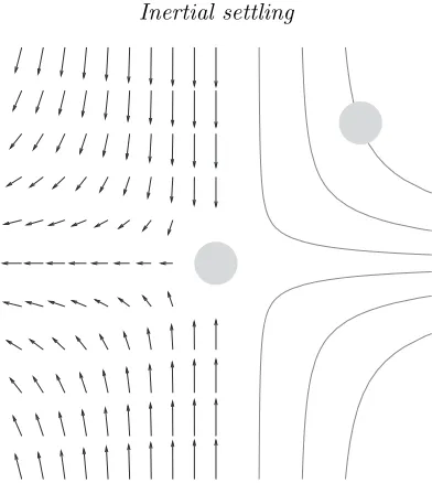
Figure 5. Schematic of inertia-induced interaction between two identical spherical particles falling in a viscous fluid.
velocity of one particle relative to the ‘reference’ particle in the frame moving with the latter (placed at the centre). Grey solid lines represent trajectories of their relative motion. This type of interaction shows the tendency toward horizontal alignment of particles during their fall and is in agreement with the previously mentioned experiments by Jayaweera et al. (1964). Of course, these arguments are valid as long as ReZ 1 (the condition ReZ−2 reduces to the less restrictive condition ReZ−1, since an intermediate outer region is absent), which is the case whenever the Stokes approximation is time independent in some co-moving coordinate frame, e.g. the settling of two identical spheres in an arbitrary spatial arrangement or the settling ofN spheres at vortices of a regular polygon in horizontal alignment. For larger separations,Z Re−1, the particles would interact via their Oseen regions and a much weaker effect on their mobility is expected. Indeed, Jayaweera et al. (1964) observed a maximum limiting separation for two equal particles settling side-by-side which decreases with increases inRe.
Note that trajectories in figure 5 have the same topology as the flow field in the overlap Oseen outer region, proportional to (A−12Ue), and, as argued by Bretherton (1964), under the limitZ−2ReZ−11, when the particles are approximated as point-like objects, their relative mobility is due to this flow and thus small oscil-lations about horizontal alignment caused by purely viscous interaction between spheres are damped by weak inertia in the long-time limit.
In comparison with the case of equal-sized particles, the solution for unequal parti-cles is also affected by the contribution from the intermediate region,r∼Re−1/2, by fluid acceleration in the vicinity of particles,∂v0/∂t, and by the inertia of the parti-cles, since their motion is unsteady. In this axisymmetric case, the stresslet strength is given in terms of a scalar functionS0 as
S0= (ee−13I)S0(Z(t)),
0 1 2 3 4 5
−0.10 −0.09 −0.08 −0.07 −0.06 −0.05
•
separation
U
1 1,
U
[image:17.612.195.407.73.208.2]1 2
Figure 6. The inertial corrections to the velocity of the unequal spheres. Solid curves, smaller particle falls ahead of the larger trailing particle; dashed curves, vice versa. Upper and lower curves correspond to the velocity of a trailing and a leading particle, respectively.
separation 10−2
10−1 100
10−3
0 0.1 0.2 0.3
10−2 10−1 100 101
Re (R−1) attraction
repulsion
separation
10−2 10−1 100 101
(a) (b)
(∂Ur0 / ∂R)R=1
−Ur1
Figure 7. The relative motion of slightly unequal spherical particles falling along the line of cen-tres in a constant gravity field. (a) (∂Ur0/∂R)R=1and−Ur1versus separation between particles’ surfaces. (b) Domains of attraction and repulsion.
equal to 1 and 1.2, respectively, and density ratio λ = 1.005. The computed iner-tial corrections to the individual particle’s velocities are plotted in figure 6 for two configurations: (i) a smaller particle falls ahead of the larger one; and (ii) a smaller particle trails after the larger one. Again, the circle at zero separation corresponds to the Oseen velocity for touching unequal spheres found by using (4.1). When the particles are of different sizes, their relative Stokes velocity isO(1) and, therefore, a small amount of inertia would only have a minor effect on their interaction dynamics. Nevertheless, when the spheres are only slightly unequal, the competition between the effect of inertia induced attraction and the gravity-induced repulsion may lead to the interesting selection of an equilibrium separation between the particles during their settling. The relative velocity,Ur, can be expanded as
Ur=Ur0(Z, R) +ReU 1
r(Z, R) +o(Re), (4.2)
where Ur0 is a quasi-stationary relative velocity and R = a1/a2 is a dimensionless radius of the leading particle.Ur0(Z, R) is positive forR >1 (when the larger particle is the leading one), whileU0
[image:17.612.113.487.259.403.2]each other. Expanding Ur0 in the vicinity of R = 1, the expression in (4.2) can be rewritten as
Ur=Re
Ur1(Z,1) +R−1 Re α(Z)
+o(Re, R−1), (4.3)
where
α(Z) = ∂U 0 r(Z, R)
∂R
R=1 .
The functionα(Z) and the contribution to the relative velocity of equal spheres due to fluid inertia,Ur1(Z,1), are plotted in figure 7aas functions of separation between particle surfaces,Z−R−1. It is obvious that if
G(Z) =−U 1 r(Z,1) α(Z) >
R−1 Re =Q,
then the relative velocity is negative and the particles are attracted. In the opposite case, the relative velocity is positive and particles are repulsed. The domains of attraction and repulsion in the plane of parameters (Q, Z −R−1) are shown in figure 7b. Equilibrium separations,Z∗, corresponding to zero relative velocity such that Q = G(Z∗) are unstable with respect to a small deviation from Z∗, i.e. for Z < Z∗ the particles would attract each other, while for Z > Z∗ they would be repelled. It is interesting to note that there is a critical valueQcr 0.09 such that, for any Q < Qcr, the inertia driven attraction dominates over the difference in particles’ weight and they are attracted for allZ.
Although in this section we address an analytically tractable case of two coaxial particles, a generalization toN interacting spheres in an arbitrary configuration is straightforward. Simulation of the weakly inertia settling of three or more particles requires numerical integration of the equations of motion (2.7) for a given value of Re. On each time-step the evolution of the particle cloud can be found from
Zi(t+ ∆t) =Zi(t) +
t+∆t
t
(Ui0(t) +ReUi1(t)) dt.
Therefore, on each time-step, one has to solve the quasi-steady Stokes problem and the O(Re) problem given by (3.28)–(3.33) and then calculate the new inertia-perturbed particle positionsZi(t+ ∆t) using the above equation.
5. Conclusions
interactions between the particles. The inertia contributions from both outer regions results in the same correction for the particle velocities, regardless of their instanta-neous configurations, while the local fluid inertia (transient and quadratic terms) in the inner region and the inertia of the particles result in distinct velocity corrections for different particles atO(Re). As anticipated in Leshanskyet al. (2003), the effect of unsteadiness of the process due to temporal change of the flow domain is restricted to O(Re) and it does not affect the instantaneous particles’ velocities at O(√Re). Moreover, it is shown that the convective Oseen terms and the local quadratic inertia terms in the vicinity of the assemblage are of the same order of magnitude as the unsteady inertia terms and, therefore, considering unsteady inertia terms alone while neglecting the quadratic inertia terms as in Feng & Joseph (1995) is not justified, at least when the typical inter-particle separation,s, is not large,Re < (a/s)2, and may lead to incorrect results.
For the classical case of a coaxial settling of two equal-sized spheres that fall with the same velocity under creeping-flow approximation, we found that non-negligible inertia leads to their approach along the line of their centres. The velocity of the leading particle is slowed down to an extent greater than that of the trailing particle. For the unequal particles, the same qualitative behaviour is obtained: the velocity of both particles decreases due to fluid inertia, while the velocity of the leading particle is slowed down to much greater extent than that of the trailing particle due to the mutual interaction. The inertia contribution to the velocity of the trailing sphere seems to be less sensitive to particles’ sizes than that of the leading one. For moderate separations between particles, the proposed asymptotic theory is in an excellent agreement with available experimental observations up toRe∼3, while for a vanishing separation distance, the inertial corrections to the particles’ velocity tend to the Oseen velocity corresponding to sedimenting touching spheres (Brenner 1961). It was also demonstrated that for slightly unequal particles that would separate when the fluid inertia is entirely neglected, the inertial attraction may compensate the difference in weight and result in their approach. In the case of exact compensation, the interplay of gravity and inertia forces results in a new stationary configuration of falling spheres, which was shown to be unstable.
To conclude, we believe that insights gained from the analysis of this special asymp-totic limit will be important in understanding the dynamics of clusters at finite Reynolds number.
O.M.L. acknowledges the support of the Israel Ministry for Immigrant Absorption.
Appendix A. Solution of an outer Oseen problem
Let us introduce a spherical coordinate system (, θ, φ), where=Rer=|ζ|, having thez-axis aligned with the direction of the gravitational acceleration,e. Making use of the axial symmetry of the far outer problem, we rewrite (3.17) in terms of the scalar stream-function, which relates to the velocity components as
V0 =−
1 2sinθ
∂Ψ0
∂θ , V 0 θ =
1 sinθ
∂Ψ0
∂ . (A 1)
Thus (3.17) produces the classical Oseen equation
E4Ψ0 =−U
cosθ ∂ ∂−
sinθ
∂ ∂θ
where
E2= ∂ 2
∂2 + sinθ
2 ∂ ∂θ
1 sinθ
∂ ∂θ
.
The solution of the Oseen equation driven by the monopole singularity at ζ = 0, according to (3.16), withF0 =F0e, is given by (van Dyke 1975)
Ψ0= F 0
4πU(1−cosθ)(1−e
−U (1+cosθ)/2
). (A 2)
Next we expand this solution in the vicinity of= 0 to obtain
Ψ0 = F 0
8π(sin
2θ+2Υ(θ)) +O(3), (A 3)
whereΥ(θ) =−Usin2θ(1 + cosθ)/4π. We rewrite (A 3) in terms of an intermediate spatial variable, and, using the definition of the stream-function (A 1), arrive at the outer limit of the velocity in intermediate region,
V(ξ, t) −εF
0·G(ξ)
8π +ε
2(F0·e)A(ρ−1ξ)
8π as|ξ| → ∞, (A 4)
whereρ=εr=|ξ|and with the radial and tangential components ofA(ρ−1ξ) given by
Aρ=−sinθ ∂Υ
∂θ and Aθ= 2 sinθΥ, respectively. Alternatively, it can be rewritten in Cartesian form as
Ai(ρ−1ξ) = 12U
ei+ 1
ρ(ejξj)ei− 1 2ρ
1− 1 ρ2(ejξj)
2
ξi
. (A 5)
References
Brady, J. F. & Bossis, G. 1988 Stokesian dynamics.A. Rev. Fluid Mech.20, 111–157.
Brenner, H. 1961 The Oseen resistance of a particle of arbitrary shape. J. Fluid Mech. 11, 604–610.
Bretherton, F. P. 1964 Inertial effects on clusters of spheres falling in a viscous fluid.J. Fluid Mech.20, 401–410.
Caflisch, R. E., Lim, C., Luke, J. H. C. & Sangani, A. S. 1988 Periodic solutions for three sedimenting spheres.Phys. Fluids 31, 3175–3179.
Durlofsky, L., Brady, J. F. & Bossis, G. 1987 Dynamic simulation of hydrodynamically inter-acting particles.J. Fluid Mech.180, 21–49.
Feng, J. & Joseph, D. D. 1995 The unsteady motion of solid bodies in creeping flows.J. Fluid Mech.303, 83–102.
Golubitsky, M., Krupa, M. & Lim, C. 1991 Time-reversibility and particle sedimentation.SIAM J. Appl. Math.51, 49–72.
Happel, J. & Brenner, H. 1965 Low Reynolds number hydrodynamics. Englewood Cliffs, NJ: Prentice Hall.
Happel, J. & Pfeffer, R. 1960 The motion of two spheres following each other in a viscous fluid.
AIChE J.6, 129–133.
Hocking, L. M. 1964 The behaviour of clusters of spheres falling in a viscous fluid. J. Fluid Mech.20, 365–400.
J´anosi, I. M., T´el, T., Wolf, D. E. & Gallas, A. C. 1997 Chaotic particle dynamics in viscous flow: the three-particle Stokeslet problem.Phys. Rev.E56, 2858–2868.
Jayaweera, K. O. L. F., Mason, B. J. & Slack, G. W. 1964 The behaviour of clusters of spheres falling in a viscous fluid.J. Fluid Mech.20, 121–128.
Kim, S. & Karrila, S. J. 1991Microhydrodynamics: principles and selected applications. Oxford: Butterworth-Heinemann.
Ladyzhenskaya, O. A. 1969 The mathematical theory of viscous incompressible flow. London: Gordon & Breach.
Leichtberg, S., Weinbaum, S., Pfeffer, R. & Gluckman, M. J. 1976 A study of unsteady forces at low Reynolds number: a strong interaction theory for the coaxial settling of three or more spheres.Phil. Trans. R. Soc. Lond.A282, 585–610.
Leshansky, A. M., Lavrenteva, O. M. & Nir, A. 2003 The leading effect of fluid inertia on the motion of rigid bodies at low Reynolds number. (Submitted.)
Lovalenti, P. M. & Brady, J. F. 1993 The hydrodynamic force on a rigid particle undergoing arbitrary time-dependent motion at small Reynolds number.J. Fluid Mech.256, 561–605. Mo, G. & Sangani, A. S. 1994 A method for computing Stokes flow interactions among spherical
objects and its application to suspensions of drops and porous materials. Phys. Fluids 6, 1637–1652.
Oseen, C. W. 1927Hydrodynamik. Leipzig: Akademische Verlagsgesellschaft.
Pozrikidis, C. 1992Boundary integral and singularity methods for linearized viscous flow. Cam-bridge University Press.
Sierou, A. & Brady, J. F. 2001 Accelerated Stokesian dynamics simulations.J. Fluid Mech.448, 115–146.
Snook, I. K., Briggs, K. M. & Smith, E. R. 1997 Hydrodynamic interactions and some new periodic structures in three particle sediments.PhysicaA240, 547–559.