R E S E A R C H
Open Access
Argentine government policies: impacts on
the beef sector
Gustavo Rossini
1*, Rodrigo García Arancibia
2and Edith Depetris Guiguet
2* Correspondence: grossini@fce.unl.edu.ar 1Applied Economic Institute of
Litoral (IECAL), National University of Litoral and Catholic University of Santa Fe, Moreno 2557, 3000 Santa Fe, Argentina
Full list of author information is available at the end of the article
Abstract
Beef is a staple food for Argentine consumers, and although the country has been a major exporter, the highest proportion of beef production is consumed in the domestic market. With rising inflation rates in the last 5 years, and given the beef prices’strong weight on the composition of the Consumer Price Index, the Argentine government began taking measures to control it. They initially forced price agreements with members of the marketing and production chain and ended up with a total ban on exports. The results were not as expected and caused serious distortions at different levels of the beef chain. This study aimed to determine whether the impact on some economic and production variables would have been different without such intervention. A VAR model was estimated in order to compare the observed behavior with intervention measures and estimated predictions with a theoretically free market.
Keywords:Argentine beef exports, VAR model, Policy impacts
Background
The agri-food sector is very important to the Argentine economy, generating almost 30% of the Gross Domestic Product (GDP) and 50% of its total exports (Obschatko 2012). The beef sector has been an outstanding component, generating 22% of the agricultural sector gross domestic production and 6% of the total manufacturing pro-duction (INDEC 2012).
Generally, around three quarters of beef production has been consumed domestically, with the remaining volumes exported. It allowed positioning the country as one of the larger exporters in the world market situation, which changed in the last years as a result of several government measures. While beef exports between the years 1995 and 2005 averaged 15% of total beef production, the participation was reduced to 7% in 2014 (MINIAGRI 2015). From being the world’s third largest beef exporter, with 775,000 tons in 2005, the country descended to the 11th place, with 197,000 tons in 2014, well behind its neighbors, Brazil, Uruguay, and Paraguay (MINIAGRI 2015; COMTRADE 2016).
In the domestic market, beef is considered a staple food and as such a key compo-nent of the family consumption basket; therefore, it monopolizes government attention both to ensure its availability to the entire population and to watch the impact it has on consumer price changes. Since beef carries a 4.5% weight in the Consumer Price
Index (CPI), the government became worried. This led it to take several improvised and abrupt short-term policy measures to keep prices under control since 2005.
Following the 2002 devaluation and economic crisis, the beef sector began a slow recovery. Initially, livestock and beef prices remained stable, but later on, a sustained domestic and foreign demand pushed them up. Domestically, beef demand got stronger basically as a result of an improvement in the population real income. Internationally, it was fueled by some emerging countries growth, large purchases by Russia and Chile, and the crisis of other suppliers from the mad cow disease. As a result, there was an excess of beef demand which was rapidly reflected into domestic prices. Nevertheless, by 2005, the exchange rate had tripled while average beef prices had only doubled (Melitsko et al. 2012).
The strong incidence on the CPI and the accelerating inflation rates moved the govern-ment to intervene actively. Initially, in March 2005, governgovern-ment carried out a price agree-ment with the private sector attempting in vain to curb the price rise; in August, it imposed a minimum slaughter weight for live animals with objective to increase the sup-ply of heavier animals; in November, the target was to restrict foreign sales, elevating export taxes to 15%, and eliminating the export reimbursements of indirect taxes (5%). In January 2006, an export registry system (ROE)1was created. The government office in charge of administering the system (ONCCA)2was given the power to extend an export authorization for each shipment, as a precondition to the custom clearance. Delays and arbitrary objections were later used as means to interfere and discourage operations. Fur-thermore, in March 2006, beef exports were initially banned for 180 days. Later on, a quantitative restriction policy was implemented, forcing beef packers to export only domestic market surpluses.
In 2007, to keep the system of“suggested maximum prices”to consumers, the govern-ment granted subsidies to feed lots to buy corn, policy which continued up to 2011 when the ONCCA was closed, under strong suspicion of corruption.
By 2010–2012, the negative effects of those measures at different levels of the beef chain were visible. For example, cattle stock dropped by more than 10 million heads between 2007 and 2012 (severe droughts and floods added significantly to this decline) and domestic cattle price increased by 300% and beef consumer price by more than 400% between 2005 and 2012 (IPCVA 2015). General inflation rate in Argentina for this period was approximately 319%3. Many cattle farms liquidated their cattle stocks and turned to soybean production, and 20% of the number of beef packers closed or suspended their businesses.
The performance did not improve much during 2013 and 2014, with the domestic market absorbing 93.6% of all beef production, the highest percentage in 53 years. Pro-duction and export continued declining, and an estimated 130 slaughter plants and 15,600 jobs disappeared4.
To essay an answer to these questions, this paper aims to estimate the difference of two different scenarios: one with actual data of what really happened and another with a simulated one without government intervention.
This paper is structured as follows. In the following section, the time series method used to estimate the model is exposed. Then, the results of the model and the esti-mated impacts of the economic policies applied to the beef sector are calculated. Finally, in the last section, conclusions and implications of the results are presented.
Methods The VAR model
Given the complexity of the beef market in Argentina, it is interesting to analyze it from a multivariate perspective. In the analysis of time series data, vector auto-regression models (VAR) have been widely used in empirical works. The VAR model was proposed by Sims (1980) as an alternative to simultaneous equation models. The VAR processes are a generalization of multivariate autoregressive models (AR), where each variable is regressed on a set of others with several lags (Hamilton 1994; Enders 2009).
Following Becketti (2013), a univariate simple model (AR) without exogenous variables can be represented as
yt ¼uþ∅1yt−1þ…þ∅pyt−pþt
compactly as
∅ð ÞL yt¼uþt
Where ytis a function of a constant (μ),ppast values oft, and a random variable εt. If we consider a vector together with endogenous variables
yt ¼
y1;t
y2;t
y3;t
: : :
yn;t
2 6 6 6 6 6 6 4
3 7 7 7 7 7 7 5
It can be modeled ofnelements as a function ofnconstant,ytpast values of the vec-torp, and a vector ofnεtrandom errors.
yt ¼uþΦ1yt−1þ… þΦpyt−pþt
In this equation,μare the elementnconstant vector
u¼
u1
u2
: : :
up
2 6 6 6 6 6 6 4
3 7 7 7 7 7 7 5
Φi¼
ϕi;11 ϕi;12 … ϕi;1n
ϕi;21 ϕi;22 … ϕi;2n
: : … :
: : … :
: : … :
ϕi;n1 ϕi;n2 … ϕi;nn 2
6 6 6 6 6 6 6 4
3 7 7 7 7 7 7 7 5
Andεtis a vector ofnelements of random errors where
E tÞ ¼0 y E t0sÞ ¼ Σ0;; tt≠¼sgs
being Σ the variance-covariance matrix. It is important to note that the elements εt could be contemporaneous correlated. Also, the VAR model can be written as a VAR withplags in a more compact way
Φð Þ ¼L I−Φ1ð ÞL −⋯−Φpð ÞL
whereΦ (L) is a matrix of polynomials in the lag operator. The number of lags to include in the VAR model is selected by some information criteria such as Akaike’s information criterion (AIC) or Schwarz’s Bayesian information criterion (SBIC). Other tests used to check the adequacy of the VAR model comprise autocorrelation in the residuals (Lagranger multiplier) and a test for normality distribution in the distur-bances (Jarque-Bera).
VAR model predictions can be performed directly, which can be one-period ahead or dynamic. In this work, more interesting results can be achieved carrying out dynamic predictions over a period ahead.
Results and discussion
Scenario with the actual evolution of selected variables
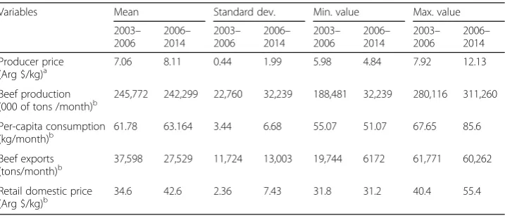
Descriptive statistics of the main variables included in the model are shown in Table 1 for periods January 2003 to March 2006 and April 2006 to May 2014. The price data were deflated to values of June 2013 using the official price index published by the Na-tional Institute of Statistical and Census from 2003 to 2006 and then the Consumer Price Index published by the National Congress of Argentina. The reason of using both indexes is because the official price index published by the National Institute of Statistical and Census became unreliable after 2007.
Cattle monthly average price was higher in the second period (Arg. $8.11/kg.) com-pared to the first one (Arg.$7.06/kg), with a difference of almost 15% between them. Monthly beef production showed similar average monthly values in both periods and per-capita monthly beef consumption just a few differences between both periods (61.78 kg/month, against 63.13 kg/month). However, there were significant differences in the average beef exports and retail domestic price for both periods. In beef exports, Argentina exported in average a 27% less in the second period when government con-trols were in place (2006–2014), and also consumer paid approximately 23% more per kilogram in that period.
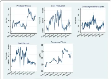
The behavior of the variables included in the VAR model is shown in Fig. 1. Altogether, they illustrate the present scenario. In all of them, it is possible to observe the significant changes that occurred in the beef sector after 2010, with declines in pro-duction, exports, and per-capita consumption. In contrast, it is observed an increase in retail and beef cattle prices.
Results of VAR model
A model VAR of five equations was set with beef cattle price, beef production, per-capita beef consumption, retail beef price, and the volume of beef exports. Taking them as the beef market most relevant variables, their interactions allow modelling the mar-ket behavior in a reasonable manner and test the impact of sectorial economic policies. At the same time, two exogenous variables were added to the model, such as beef cuts’ prices received by exporters and soybean price. The first was taken as exogenous
Table 1Descriptive statistics
Variables Mean Standard dev. Min. value Max. value
2003– 2006
2006– 2014
2003– 2006
2006– 2014
2003– 2006
2006– 2014
2003– 2006
2006– 2014
Producer price (Arg $/kg)a
7.06 8.11 0.44 1.99 5.98 4.84 7.92 12.13
Beef production
(000 of tons /month)b 245,772 242,299 22,760 32,239 188,481 32,239 280,116 311,260
Per-capita consumption
(kg/month)b 61.78 63.164 3.44 6.68 55.07 51.07 67.65 85.6
Beef exports (tons/month)b
37,598 27,529 11,724 13,003 19,744 6172 61,771 60,262
Retail domestic price
(Arg $/kg)b 34.6 42.6 2.36 7.43 31.8 31.2 40.4 55.4
a
Liniers cattle market
b
because Argentina is considered a price-taker participant in the international beef mar-ket. In turn, the soybean price was included because soybean production is seen as an alternative to livestock production in Argentina, competing for resources such as land and capital. Other exogenous variables were initially included in the model, for example, chicken and corn prices, with no significant differences in the results. In con-sequence, they were excluded in order to have a more parsimonious model.
The variables were tested for unit roots. Three types of tests are shown in Table 2. The producer price, per capita consumption and beef export variables were stationaries according to the tests used. However, beef production and the average retail price only showed evidence of being stationary at the 10% level of statistical significance. Conse-quently, a VAR model with five variables was estimated by the given sample size.
Table 2Unit root tests
Variables Dickey-Fuller Phillips-Perron KPSS
Producer price −3.637**
(2.96)
−2.89* (2.96)
0.102*** (0.146)
Beef production −1.939
(2.96) −
2.318* (2.96)
0.149** (0.146)
Per-capita consumption −2.778*
(2.96) −
4.930*** (2.96)
0.16** (0.146)
Export beef −2.246*
(2.96) −
3.881** (2.96)
0.157** (0.146)
Retail beef price −2.596*
(2.96)
2.449* (2.96)
0.188** (0.146)
Note: Critical values at 5% level of significance in parenthesis
*, **, ***Statistically significant at 10, 5, and 1% levels
4 6 8 10 12 Arg $/kg
2002m12004m12006m12008m12010m12012m12014m1 Producer Prices
200000
250000
300000
Tons/month
2002m12004m12006m12008m12010m12012m12014m1 Beef Production 50 60 70 80 90 kgs/person
2002m12004m12006m12008m12010m12012m12014m1 Consumption Per-Capita 0 20000 40000 60000 Tons/month
2002m12004m12006m12008m12010m12012m12014m1 Beef Exports 20 30 40 50 60 Arg $/Kg 2002m12004m12006m12008m12010m12012m12014m1 Consumer Prices
The number of lags in the VAR model was determined according to different selec-tion criteria. A model with four lags responded to the informaselec-tion Akaike (AIC) and information of Quinn (HQIC) criterion and only three lags to the Schwarz Bayesian (SBIC) criterion. On this basis, a model with three lags was estimated, since it ensured that residuals were uncorrelated, saving degrees of freedom and obtaining a more parsi-monious model.
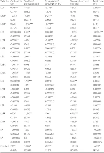
The coefficients of the VAR model for the period January 2003 to March 2006 are shown in Table 3. A total of 18 coefficients were estimated in the system, including the exogenous variables. The coefficients showed a stationary process since the eigenvalues of the estimated VAR model were located inside the unit circle.
Many of the VAR model coefficients were not statistically significant. Nonetheless, re-ducing the lags to one or two generated a model with correlated residuals, and the Jarque-Bera test rejected the null hypothesis of normal disturbances on residuals. Test-ing the lags in each equation of the VAR model, it was found that the first lag in the per-capita consumption equation was not significant, as well as the third lag in the pro-ducer price and export beef equations. However, lags were significant when the VAR model as a whole was considered7.
The test of the Lagrange multiplier for residuals indicated no correlation at the 1% level (Table 4).
Moreover, the Jarque-Bera test did not reject the null hypothesis of normal distur-bances in all residuals (Table 5).
Based on the estimated coefficients of VAR model for the period 2003–2006, predic-tions were made in order to compare with observed values. Therefore, possible losses or gains generated by the effect of intervention measures were calculated between April 2006 and May 2014.
Scenario with predicted results Predictions based on VAR model
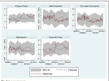
Predictions about the price of the beef cattle started in April 2006, after one of the first significant measures imposed by the government banning beef exports for 180 days; prices were close to those observed. Later on, the model did not capture the significant rise that took place in the cattle price, although at the end of the period, the estimated values were very close to those observed. The gray area shows 95% confidence intervals of dynamic predictions. The observed prices in general remained within this area, ex-cept for the unusual rise after the cattle stock liquidation in previous years, which was exacerbated by a severe flood in the year 2007 and drought in 2009. Forecasts also imply that if the market had acted more freely, producer prices of beef cattle would had been more stable.
Table 4Lagrange multiplier test for residuals
Lags Chi2
Df Prob > chi2
1 25.45 25 0.437
2 29.66 25 0.236
Note H0: no autocorrelation at lag order
Table 3Coefficients of the VAR model
Variables Cattle prices (CP)
Total beef production (BP)
Per-capita beef consumption (BC)
Volume of exported beef (BE)
Retail prices (RP)
L.CP 0.946*** −7927 −3.176* −2701 0.892***
(0.171) (8152) (1.894) (3740) (0.344)
L2.CP −0.353 16,641 6.424*** 4620 −0.453
(0.22) (10,514) (2.443) (4824) (0.443)
L3.CP 0.0204 −2763*** −6.774*** −6008 0.147
(0.167) (7992) (1.857) (3667) (0.337)
L.BP 0.00000009 0.658* 0.000003 −0.155 −0.0004***
(0.000007) (0.368) (00000.8) (0.169) (0.00001)
L2.BP 0.00002** −0.261 −0.00005 −0.0782 −0.00001
(0.000009) (0.45) (0.000105) (0.207) (0.00002)
L3.BP 0.000004 0.570* 0.000206*** 0.201 0.000004
(0.000006) (0.299) (0.000007) (0.137) (0.00001)
L.BC −0.00651 2905** −0.0913 1024* 0.117**
(0.0241) (1152) (0.268) (0.528) (0.0486)
L2.BC −0.0515* 899.3 0.114 943.4 0.0835
(0.0299) (1429) (0.332) (655.8) (0.0603)
L3.BC −0.0269 −1181 −0.221 −927.9* 0.0643
(0.0227) (1086) (0.252) (498.4) (0.0458)
L.BE 0.0000008 1.726*** 0.00001 0.508** 0.00003
(0.00001) −0.541 (0.000126) (0.248) (0.00002)
L2.BE −0.00002 0.872 −0.000157 0.507 0.000005
(0.00002) (0.745) (0.000173) (0.342) (0.00003)
L3.BE −0.00002 −0.651 −0.00006 −0.248 0.00002
(0.00002) (0.651) (0.000151) (0.299) (0.00003)
L.RP −0.106 −6687 −0.689 −3736* 1.040***
(0.0922) (4408) (1.024) (2.022) (0.186)
L2.RP 0.206* 11,540** 1.764 6.966*** −0.282
(0.121) (5.794) (1.346) (2.658) (0.244)
L3.RP −0.0618 −4.131 −1.145 −2826* 0.185
(0.0784) (3.744) (0.87) (1718) (0.158)
EP −0.00003 1.089 0.00036 −0.333 −0.00003
(0.00002) (1.126) (0.000262) (0.517) (0.00004)
SP −0.000009 0.9 0.000459 −3.625 −0.000401
(0.000186) (8.899) (0.00207) (4.083) (0.000375)
Constant 2.159 170.27* 57.29** −12.174 −6.936*
(2.053) (98,089) (22.79) (45,003) (4.136)
The model predicted stable values of per-capita beef consumption, differing from those observed, particularly in regard to its variability. In general, consumption fore-casts ranged from 52 kg per-capita to 70 kg per capita, showing a slight decreasing trend.
With respect to average retail prices of beef cuts, there are two distinctive periods. Before 2010, the model predicted prices slightly higher than those observed, while after 2010, retail prices were lower. In summary, predicted prices remained with a few changes, with a slight upward trend.
Beef export forecasts showed higher values than those actually observed. Between 2006 and up to mid-2009, the exported volumes were slightly higher, but in general close to those observed. However, the exported volumes showed a wider difference for the period after 2010.
A more detailed analysis of losses and gains on exports, domestic consumption, and producer prices is presented in the next sections.
Table 5Jarque-Bera test
Equation Chi2 dfprob > chi2
Prod. price 0.455 0.7964
Beef production 0.680 0.7116
Per-capita consumption 0.956 0.6199
Beef exports 1.180 0.5543
Retail beef price 0.277 0.8705
All 3.549 0.9654
Note H0: normal disturbances
0
5
10
15
100000
200000
300000
400000
40
60
80
100
-50000
0
50000
100000
20
30
40
50
60
2006m1 2008m1
2010m1 2012m1
2014m1
2006m1 2008m1
2010m1 2012m1
2014m1 2006m1 2008m1
2010m1 2012m1
2014m1
Producer Prices Beef Production Per-capita Consumption
Beef Exports Consumer Prices
95% CI Forecast
Observed
Losses and gains from the intervention in the beef sector
Domestic consumption
One of the objectives defined by the government intervention was to keep low domes-tic prices, pardomes-ticularly for food items. However, results from the model showed that it had a low impact on retail beef price. The average observed retail price was Arg. $42.6 per kilogram, while the predicted without government intervention was Arg. $41.8 per kilogram. This suggests that even with drastic measures such as the barriers and bans to exports, government failed to keep low beef retail price.
At the same time, an estimation of what it would have been the values paid by con-sumers given the average monthly prices and the monthly consumption in the domes-tic market (total production minus total exports) without government measures was done. Figure 3 shows that actual consumer expenditure on beef compared to the pre-dicted values was lower in the early years of imposed restrictions but higher after the year 2010.
The sum of observed and predicted total consumer expenditures in the domestic market yielded a total value of Arg. $ 14,249 million (US$ 2673 million8). It means that the consumer losses were very high, and it confirmed that agricultural policies applied to keep low domestic prices did not reach their objective.
Beef exports
The difference between beef exports and model predictions under government inter-vention for the period 2006–2013 was approximately 1.5 million of tons. This means an average of 180,000 tons per year or about 15,000 tons per month. Of those, 1.14 million of tons (252,325 tons a month on average) export losses corresponded to the period with a stronger government intervention (2010–2014). Valued at prices received by exporters, the value loss of entire period reached US$ 8000 million, of which US$ 6.800 million belonged to 2010–2014.
Monthly beef exports predicted and observed are showed in Fig. 4, as well as the evolu-tion of average prices. Losses have been higher after 2010 when the government only authorized exports for approximately 20,000 ton per month, despite prevailing good prices in the international beef markets.
4000
5000
6000
7000
8000
Million $ Arg
2006m1 2008m1 2010m1 2012m1 2014m1
Consumer Expenditure Forecasted Consumer Expenditure
Producer cattle prices
Predicted cattle prices were higher than observed ones before 2010 and lower in the period 2010–2014. Before 2010, a strong cattle supply pushed cattle prices down, and after 2010, the opposite occurred, cattle supply was reduced, increasing prices.
In order to examine whether producers income has been impacted by the interven-tionist policies, effective and predicted income values were calculated (total production by cattle prices). For the period 2006–2014, the predicted producer income loss was Arg. $1470 million, which represented almost US$ 275 million. Figure 5 shows a clear difference between the real income and the predicted value by the VAR model before and after 2010. In the first period, the cattle producer sector transferred incomes to other sectors in the production and marketing chain; with the interventionist policies, cattle prices and producer income have been lower than without them. In the second period, real cattle prices increased more than predicted and so did producers income.
Evaluation of VAR forecast
In order to evaluate dynamic forecasts from VAR, we compared the performance of VAR forecasts with predictions generated by other procedures. Three techniques are used to compare to VAR forecasts9: (a) simple mean of the variables, (b) predictions
3000
4000
5000
6000
7000
8000
US$/Ton.
0
20000
40000
60000
Tons/month
2006m1 2008m1 2010m1 2012m1 2014m1
Forecast Observed US$/Ton.
Fig. 4Beef export losses
-20000
-10000
0
10000
20000
Arg $ Million
2006m1 2008m1 2010m1 2012m1 2014m1
from a random walk model, and (c) forecast provided by independent univariate time-series model for each variable of the model (Becketti 2013).
In Table 6, it is displayed the root mean of squared error (RMSE) obtained from pseudo out-of-sample forecasts for each of these methods and for the five endogenous variables of the VAR model. In general, the VAR forecast is an improvement on forecast techniques, particularly compared with univariate time-series models. For producer price, the relative performance of the VAR worsen as the forecast horizon increases, and for two-step-ahead forecast, for example, the RMSE of VAR forecast is 47% smaller than the RMSE of the mean forecast, 34% larger than the RMSE of random walk fore-cast, and 46% smaller than the RMSE of the univariate AR forecast.
Conclusions
The objective of this paper has been to investigate the impacts of government policies on the beef sector in Argentina, particularly evaluating the effects of those measures over some variables such as beef production, producer prices, beef exports, consumer prices, and domestic consumption.
Table 6Root mean of squared error (RMSE) of VAR forecasts compared with other prediction methods
Method % Improvement
Producer price
Horizon Mean RW AR VAR Mean RW AR
3 2.57 1.02 2.55 1.37 47 −34 46
6 2.65 1.39 2.63 1.97 26 −42 25
9 2.73 1.84 2.74 2.18 20 −19 20
12 2.81 2.21 2.85 2.35 16 −6 18
Beef production
3 34,128.54 24,523.4 31,307.19 24,693.97 28 −1 21
6 33,671.6 30,892.22 31,041.01 34,135.24 −1 −10 10
9 33,508.45 31,404.72 30,529.84 34,552.06 −3 −10 −13
12 33,811.04 33,434.45 30,769.51 32,812.82 3 2 −7
Per-capita consumption
3 6.64 5.05 6.22 4.46 33 12 28
6 6.47 5.52 6.11 6.13 5 −11 0
9 6.46 6.04 6.1 6.72 −4 −11 −10
12 6.43 7.04 6.13 7.18 −12 −2 −17
Beef exports
3 13,486.92 9729.23 12,921.88 10,950.07 19 −13 15
6 13,734.65 11,689.7 13,195.46 14,059.92 −2 −20 −7
9 14,412.9 13,930.08 13,899.11 14,090.93 2 −1 −1
12 14,915.21 14,508.85 14,392.13 12,692.69 15 13 12
Retail beef price
3 11.21 4.54 11.04 4.45 60 2 60
6 11.4 5.94 11.24 7.32 36 −23 35
9 11.73 6.23 11.57 8.82 25 −42 24
12 12.14 7.63 12.05 9.06 25 −19 25
The model used in this work has allowed estimating the theoretical losses generated by government economic measures that influenced beef exports, beef production, pro-ducer income, and prices paid by consumers.
After the 2002 crisis which affected the Argentine economy, the government gradually intensified its intervention in the beef sector. Its main objective was to keep retail prices low and, indirectly, its incidence in the CPI. Following years of explicit as well as disguised control measures, a drop in cattle stock occurred, by almost 10 million head, as well as in beef exports, while beef consumer price also increased.
This study revealed that with less government intervention, beef production would have been larger as well as the proportion exported, and producer and consumer prices would have been more stable for the analyzed period. This kind of government inter-vention has had important economic consequences, such as the drop in exports. The model estimated losses of 1.5 million tons of beef exports, with an estimated value of 8000 million dollars between the years 2010 and 2014. Decreases have also been found in producer income and consumer expenditures.
Lastly, there were many others losses which have not been quantified in this work. For example, by non-fulfillment of contracts with buyers abroad, such as the Hilton Quota, reputation is a reliable supplier in the international market; jobs lost for meatpackers from a reduction in volumes processed, canceled investments for the negative prospective, reduction in by-products manufactured such as leather articles, and among others.
Elections were held in Argentina at the end of 2015, and the new government has adopted some economic and political measures for the development of the agri-food sector. These measures included devaluation of the argentine peso, elimination of the export taxes, and other measures that regulated most of the agricultural exports. Therefore, beef production is expected to recover from the erroneous path of the last years and to hold a sustainable growth pattern in the future.
Endnotes 1
ROE was the registration affidavits for the sales of agricultural products abroad, established by the Argentine government with the objective to control agricultural exports.
2
National Office of Agricultural Trade Control (ONCCA) was a government agency for ensuring compliance with trade rules by operators involved in the market of cattle, meats, grains, and dairy products, in order to ensure transparency and fairness in the development of the agro-food sector, throughout the territory of the Republic of Argentina. It was dissolved by a presidential decree in February 2011.
3
Inflation rate published by the National Congress from the period 2002–2012 4
http://en.mercopress.com/2013/05/21/argentina-absorbs-93-of-beef-production-exports-tumble-behind-paraguay
5
The largest cattle market auction in Argentina 6
Data set available from the author upon request 7
Lags of the VAR model were tested with the STATA commandwarwle, proposed by Becketti (2013).
8
Average exchange rate (peso-dollar ) for the whole period was 3.73 Arg.$/dollar 9
The STATA command varbench proposed by Becketti (2013) was used to evaluate
Acknowledgements
This research was supported by funding of National University of Litoral, Argentina, Project CAID 0416, and funding of Catholic University of Santa Fe.
Authors’contributions
GR conceived the study, collected the data, and estimated the econometric model. EDG and GR drafted the manuscript, and RGA read and made suggestions of the manuscript. All authors read and approved the final manuscript.
Competing interests
The authors declare that they have no competing interests.
Author details
1Applied Economic Institute of Litoral (IECAL), National University of Litoral and Catholic University of Santa Fe, Moreno
2557, 3000 Santa Fe, Argentina.2Applied Economic Institute of Litoral (IECAL), National University of Litoral, Moreno 2557, Santa Fe 3000, Argentina.
Received: 25 February 2016 Accepted: 28 December 2016
References
Becketti S (2013) Introduction to time series using Stata. Stata Press, Lakeway Drive, College Station, Texas COMTRADE (United Nations) (2016) Database. http://comtrade.un.org/data/
Enders W (2009) Applied econometric times series. Wiley, Hoboken, New Jersey Hamilton J (1994) Time series analysis. Princeton University Press, Princenton, New Jersey
Instituto de Promoción de la Carne Vacuna Argentina (2015) Estadísticas mensuales. http://www.ipcva.com.ar/ estadisticas. Accessed 5 Sept 2015
Instituto Nacional de Estadísticas y Censos (INDEC) (2012) Agregados macroeconómicos. http://www.indec.gob.ar/ nivel4_default.asp?id_tema_1=3&id_tema_2=9&id_tema_3=47
Melitsko S, Domínguez A, y Anchorena J (2012) Historia de un fracaso: política de carne vacuna, 2005-2013. Documento de trabajo fundación Pensar, DT012. http://www.fce.austral.edu.ar/aplic/webSIA/webSIA2004.nsf/ 6905fd7e3ce10eca03256e0b0056c5b9/6884859bae2dd1c603257d740074a1cc/$FILE/CarnevacunaArgentinafracaso. pdf. Accessed 10 Sept 2015
Ministerio de Agroindustria de Argentina (MINIAGRI) (2015) Ministerio de Agroindustria de Argentina. Indicadores bovinos anuales 1995-2015. http://www.agroindustria.gob.ar/sitio/areas/bovinos/informes/indicadores/_archivos// 000001_Indicadores/000003-Indicadores%20bovinos%20anuales%201990-2015.pdf. Accessed 26 Sept 2016 Obschatko E (2012) El sector agroalimentario argentino como motor del crecimiento.http://www.iica.int/Esp/regiones/
sur/argentina/Documentos%20de%20la%20Oficina/Cam-Arg-Hol-2013-Alimentar-el-futuro.pdf. Accessed 15 Sept 2015 Sims C (1980) Macroeconomics and reality. Econometrica 48:1–48
Submit your manuscript to a
journal and benefi t from:
7Convenient online submission 7Rigorous peer review
7Immediate publication on acceptance 7Open access: articles freely available online 7High visibility within the fi eld
7Retaining the copyright to your article