Online Learning to Rank with Top-k Feedback
Sougata Chaudhuri 1 [email protected]
Ambuj Tewari 1,2 [email protected]
Department of Statistics 1
Department of Electrical Engineering and Computer Science2
University of Michigan Ann Arbor, MI 48109, USA
Editor:Alexander Rakhlin
Abstract
We consider two settings of online learning to rank where feedback is restricted to top ranked items. The problem is cast as an online game between a learner and sequence of users, over T rounds. In both settings, the learners objective is to present ranked list of items to the users. The learner’s performance is judged on the entire ranked list and true relevances of the items. However, the learner receives highly restricted feedback at end of each round, in form of relevances of only the top k ranked items, where k m. The first setting isnon-contextual, where the list of items to be ranked is fixed. The sec-ond setting iscontextual, where lists of items vary, in form of traditional query-document lists. No stochastic assumption is made on the generation process of relevances of items and contexts. We provide efficient ranking strategies for both the settings. The strategies achieveO(T2/3) regret, where regret is based on popular ranking measures in first setting and ranking surrogates in second setting. We also provide impossibility results for certain ranking measures and a certain class of surrogates, when feedback is restricted to the top ranked item, i.e. k= 1. We empirically demonstrate the performance of our algorithms on simulated and real world data sets.
Keywords: Learning to Rank, Online Learning, Partial Monitoring, Online Bandits, Learning Theory
1. Introduction
Learning to rank (Liu, 2011) is a supervised machine learning problem, where the output space consists ofrankingsof objects. Most learning to rank methods are based on supervised batch learning, i.e., rankers are trained on batch data in an offline setting. The accuracy of a ranked list, in comparison to the actual relevance of the documents, is measured by various ranking measures, such as Discounted Cumulative Gain (DCG) (J¨arvelin and Kek¨al¨ainen, 2000), Average Precision (AP) (Baeza-Yates and Ribeiro-Neto, 1999) and others.
Collecting reliable training data can be expensive and time consuming. In certain appli-cations, such as deploying a new web app or developing a custom search engine, collecting large amount of high quality labeled data might be infeasible (Sanderson, 2010). Moreover, a ranker trained from batch data might not be able to satisfy rapidly changing user needs and preferences. Thus, a promising direction of research is development of online ranking
c
systems, where a ranker is updated on the fly. One type of online ranking models learns from implicit feedback inferred from user clicks on ranked lists (Hofmann et al., 2013). However, there are some potential drawbacks in learning from user clicks. It is possible that the system is designed for explicit ratings but not clicks. Moreover, a clicked item might not actually be relevant to the user and there is also the problem of bias towards top ranked items in inferring feedback from user clicks (Joachims, 2002).
We develop models for online learning of ranking systems, from explicit but highly restricted feedback. At a high level, we consider a ranking system which interacts with users over a time horizon, in a sequential manner. At each round, the system presents a ranked list ofmitems to the user, with the quality of the ranked list judged by the relevance of the items to the user. The relevance of the items, reflecting varying user preferences, is encoded as relevance vectors. The system’s objective is to learn from the feedback it receives and update its ranker over time, to satisfy as many users as possible. However, the feedback that the system receives at end of each round is not the full relevance vector, but relevance of only the top k ranked items, where k m (typically, k = 1 or 2). We consider two problem settings under the general framework: non-contextual andcontextual. In the first setting, we assume that the set of items to be ranked are fixed (i.e., there are no context on items), with the relevance vectors varying according to users’ preferences. In the second setting, we assume that set of items vary, as traditional query-document lists. We highlight two motivating examples for such feedback model, encompassingprivacy concerns and economic and user-burden constraints.
Privacy Concerns: Assume that a medical company wants to build an app to suggest activities (take a walk, meditate, watch relaxing videos, etc.) that can lead to reduction of stress in a certain highly stressed segment of the population. The activities do not have contextual representation and are fixed over time. Not all activities are likely to be equally suitable for everyone under all conditions since the effects of the activities vary depending on the user attributes like age & gender and on the context such as time of day & day of week. The user has liberty to browse through all the suggested activities, and the company would like the user to rate every activity (may be on an 1−5 scale), reflecting the relevances, so that it can keep refining its ranking strategy. However, in practice, though the user may scan through all suggested activities and have a rough idea about how relevant each one is to her; she is unlikely to give feedback on the usefulness (relevance) of every activity due to privacy concerns and cognitive burden. Hence, in exchange of the user using the app, the company only asks for careful rating of the top 1 or 2 ranked activities. The apps performance would still be based on the full ranked list, compared to the implicit relevance vector that the user generates, but it gets feedback on the relevances of only top 1 or 2 ranked activities.
each suggestion, unless the company provides some economic incentives to do so. Though the company needs high quality feedback on each suggestion to keep refining the ranking strategy, it cannot afford to give incentives due to budget constraints. Similar to the first example, the company only asks, and possibly pays, for rating on the top 1 or 2 ranked suggestions, in lieu of using the app, but its performance is judged on the full ranked list and implicit relevance vector.
We cast the online learning to rank problem as an online game between a learner and an adversary, played over time horizonT. That is, we do not make anystochastic assumption on the relevance vector generation process or the context (features) generation process (in the second problem setting). The adversary is considered to beoblivious, i.e., an adversary who generates moves without knowledge of the learner’s algorithm. We separately discuss the two problem settings, and our contributions in each, in greater details.
1.1 Non-contextual setting
Existing work loosely related to ranking of a fixed set of items to satisfy diverse user preferences (Radlinski et al., 2008, 2009; Agrawal et al., 2009; Wen et al., 2014) has focused on learning an optimal ranking of a subset of items, to be presented to an user, with performance judged by a simple 0-1 loss. The loss in a round is 0 if among the top k
(out of m) items presented to a user, the user finds at least one relevant item. All of the work falls under the framework ofonline bandit learning. In contrast, our model focuses on optimal ranking of the entire list of items, where the performance of the system is judged by practical ranking measures like DCG and AP. The challenge is to decide when and how efficient learning is possible with the highly restricted feedback model. Theoretically, the top k feedback model is neither full-feedback nor bandit-feedback since not even the loss (quantified by some ranking measure) at each round is revealed to the learner. The appropriate framework to study the problem is that of partial monitoring (Cesa-Bianchi et al., 2006). A very recent paper shows another practical application of partial monitoring in the stochastic setting (Lin et al., 2014). Recent advances in the classification of partial monitoring games tell us that the minimax regret, in an adversarial setting, is governed by a (two-class) property of the loss and feedback functions, called global observability and local observability (Bartok et al., 2014; Foster and Rakhlin, 2012).
Our contributions: We instantiate these general observability notions for our
prob-lem with top 1 (k = 1) feedback. We prove that, for some ranking measures, namely
Precision@n, with O(mlogm) time spent per step. Moreover, the regret of our efficient algorithm has a logarithmic dependence on number of learner’s actions (i.e., polynomial dependence on m), whereas the generic algorithm has a linear dependence on number of actions (i.e., exponential dependence onm).
For several measures, their normalized versions are also considered. For example, the normalized versions of PairwiseLoss, DCG and Precision@n are called AUC (Cortes and Mohri, 2004), NDCG (J¨arvelin and Kek¨al¨ainen, 2002) and AP respectively. We show an unexpected result for the normalized versions: they do not admit sub-linear regret algo-rithms with top 1 feedback. This is despite the fact that the opposite is true for their unnormalized counterparts. Intuitively, the normalization makes it hard to construct an unbiased estimator of the (unobserved) relevance vectors. We are able to translate this intuitive hurdle into a provable impossibility.
We also present some preliminary experiments on simulated data sets to explore the performance of our efficient algorithm and compare its regret to its full information coun-terpart.
1.2 Contextual Setting
The requirement of having a fixed set of items to rank, in the first part of our work, somewhat limits practical applicability. In fact, in the classic multi-armed bandit problem, while non-contextual bandits have received a lot of attention, the authors Langford and Zhang (2008) mention that “settings with no context information are rare in practice”. The second part of our work introduces context, by combining query-level ranking with the explicit but restricted feedback model. At each round, the adversary generates a document list of lengthm, pertaining to a query. The learner sees the list and produces a real valued score vector to rank the documents. We assume that the ranking is generated by sorting the score vector in descending order of its entries. The adversary then generates a relevance vector but, like in the non-contextual setting, the learner gets to see the relevance of only the topkitems of the ranked list. The learner’s loss in each round, based on the learner’s score vector and the full relevance vector, is measured by some continuous ranking surrogates. We focus on continuous surrogates, e.g., the cross entropy surrogate in ListNet (Cao et al., 2007) and hinge surrogate in RankSVM (Joachims, 2002), instead of discontinuous ranking measures like DCG, or AP, because the latter lead to intractable optimization problems in the query-documents setting. Just like in the non-contextual setting, we note that the top
k feedback model is neither full feedback nor bandit feedback models. The problem is an instance of partial monitoring,extended to a setting with side information (documents list) and aninfinite set of learner’s moves (all real valued score vectors). For such an extension of partial monitoring there exists no generic theoretical or algorithmic framework to the best of our knowledge.
convex surrogates considered are from three major learning to ranking methods: squared loss from a pointwise method (Cossock and Zhang, 2008), hinge loss used in the pairwise RankSVM (Joachims, 2002) method, and (modified) cross-entropy surrogate used in the listwise ListNet (Cao et al., 2007) method. The non-convex surrogate considered is the
SmoothDCG surrogate (Chapelle and Wu, 2010). For the three convex surrogates, we
establish anO(T2/3) regret bound.
The convex surrogates we mentioned above are widely used but are known to fail to be calibrated with respect to NDCG (Ravikumar et al., 2011). Our second contribution is to show that for the entire class of NDCG calibrated surrogates, no online algorithm can have sub-linear (in T) regret with top 1 feedback, i.e., the minimax regret of an online game for any NDCG calibrated surrogate is Ω(T). The proof for this result relies on exploiting a connection between the construction of optimal adversary strategies for hopeless finite action partial monitoring games (Piccolboni and Schindelhauer, 2001) and the structure of NDCG calibrated surrogates. We only focus on NDCG calibrated surrogates for the impos-sibility results since no (convex) surrogate can be calibrated for AP and ERR (Calauzenes et al., 2012). This impossibility result is the first of its kind for a natural partial monitoring problem with side information when the learner’s action space is infinite. Note, however, that there does exist work on partial monitoring problems with continuous learner actions, but without side information (Kleinberg and Leighton, 2003; Cesa-Bianchi et al., 2006), and vice versa (Bart´ok and Szepesv´ari, 2012; Gentile and Orabona, 2014).
We apply our algorithms on benchmark ranking data sets, demonstrating the ability to efficiently learn a ranking function in an online fashion, from highly restricted feedback.
The rest of the paper is divided into the following sections. Section 2 and its sub-sections detail the notations, definitions and technicalities associated with online ranking with restricted feedback in the non-contextual setting. Section 3 and its subsections detail the notations, definitions and technicalities associated with online ranking with restricted feedback in the contextual setting. Section 4 demonstrates the performance of our algo-rithms on simulated and commercial data sets. Section 5 discusses open questions and future directions of research.
2. Online Ranking with Restricted Feedback- Non Contextual Setting
All proofs not in main text are in Appendix A.
2.1 Notation and Preliminaries
The fixed m items to be ranked are numbered {1,2, . . . , m}. A permutation σ gives a mapping from ranks to items and its inverse σ−1 gives a mapping from items to ranks. Thus, σ−1(i) = j means item i is placed at position j while σ(i) = j means item j is placed at position i. The supervision is in form of a relevance vector R ={0,1, . . . , n}m,
representing relevance of each document to the query. If n = 1, the relevance vector is binary graded. For n >1, relevance vector is multi-graded. R(i) denotes ith component of R, i.e., relevance of item i. The subscript t is exclusively used to denote time t. We denote {1, . . . , n} by [n]. The learner can choose fromm! actions (permutations) whereas nature/adversary can choose from (n+ 1)m outcomes (when there are n relevance levels,
actions) as σi (resp. adversary’s ith action as Ri). Note that σ−1i simply means that we
are viewing permutationσi as mapping from items to ranks. Also, a vector can be row or
column vector depending on context.
At round t, the learner outputs a permutation (ranking) σt of the objects (possibly
using some internal randomization, based on feedback history so far), and simultaneously, adversary generates relevance vector Rt. The quality of σt is judged against Rt by some
ranking measure RL. Crucially, only the relevance of the top k ranked objects are revealed to the learner at end of roundt. Thus, the learner gets to know neitherRt(full information
problem) norRL(σt, Rt) (bandit problem). The objective of the learner is to minimize the
expected regret with respect to best permutation in hindsight:
Eσ1,...,σT
" T X
t=1
RL(σt, Rt)
#
−min
σ T
X
t=1
RL(σ, Rt). (1)
When RLis a gain, not loss, we need to negate the quantity above. The worst-case regret of a learner strategy is its maximal regret over all possible choices of R1, . . . , RT. The minimax regret is the minimal worst-case regret over all learner strategies.
2.2 Ranking Measures
We consider ranking measures which can be expressed in the form f(σ)·R, where the function f : Rm → Rm is composed of m copies of a univariate, monotonic, scalar
val-ued function. Thus, f(σ) = [fs(σ−1(1)), fs(σ−1(2)), . . . , fs(σ−1(m))], where fs :R → R.
Monotonic (increasing) means fs(σ−1(i))≥fs(σ−1(j)), whenever σ−1(i)> σ−1(j). Mono-tonic (decreasing) is defined similarly. The following popular ranking measures can be expressed in the formf(σ)·R.
PairwiseLoss & SumLoss: PairwiseLoss is restricted to binary relevance vectors and defined as:
P L(σ, R) =
m
X
i=1 m
X
j=1
I(σ−1(i)< σ−1(j))I(R(i)< R(j))
PairwiseLoss cannot be directly expressed in the form of f(σ)·R. Instead, we consider
SumLoss, defined as:
SumLoss(σ, R) =
m
X
i=1
σ−1(i)R(i)
SumLoss has the formf(σ)·R, wheref(σ) =σ−1. It has been shown by Ailon (2014) that regret under the two measures are equal:
T
X
t=1
P L(σt, Rt)− T
X
t=1
P L(σ, Rt) = T
X
t=1
SumLoss(σt, Rt)− T
X
t=1
SumLoss(σ, Rt). (2)
Discounted Cumulative Gain: DCG is a gain function which admits non-binary relevance vectors and is defined as:
DCG(σ, R) =
m
X
i=1
and becomes Pm
i=1
R(i)
log2(1+σ−1(i)) forR(i) ∈ {0,1}. Thus, for binary relevance, DCG(σ, R)
has the formf(σ)·R, wheref(σ) = [log 1
2(1+σ−1(1)),
1
log2(1+σ−1(2)), . . . ,
1
log2(1+σ−1(m))].
Precision@n Gain: Precision@n is a gain function restricted to binary relevance and is defined as
P recision@n(σ, R) =
m
X
i=1
I(σ−1(i)≤n)R(i)
Precision@ncan be written as f(σ)·R where f(σ) = [I(σ−1(1)< n), . . . , I(σ−1(m)< n)]. It should be noted that forn=k(i.e., when feedback is on topnitems), feedback is actually the same as full information feedback, for which efficient algorithms already exist (Kalai and Vempala, 2005).
Normalized measures are not of the form f(σ)·R: PairwiseLoss, DCG and Precision@n are unnormalized versions of popular ranking measures, namely, Area Under Curve (AUC), Normalized Discounted Cumulative Gain (NDCG) and Average Precision (AP) respectively. None of these can be expressed in the formf(σ)·R.
NDCG: NDCG is a gain function, admits non-binary relevance and is defined as:
N DCG(σ, R) = 1
Z(R)
m
X
i=1
2R(i)−1 log2(1 +σ−1(i))
and becomesZ(R)1 Pm
i=1
R(i)
log2(1+σ−1(i)) forR(i)∈ {0,1}. HereZ(R) = max
σ
Pm
i=1 2 R(i)−1
log2(1+σ−1(i))
is the normalizing factor (Z(R) = max
σ
Pm
i=1
R(i)
log2(1+σ−1(i)) for binary relevance). It can be
clearly seen thatN DCG(σ, R) =f(σ)·g(R), wheref(σ) is same as in DCG butg(R) = Z(R)R is non-linear in R.
AP: Average Precision is a gain function, restricted to binary relevance and is defined as:
AP(σ, R) = 1
kRk1 m X i=1 P j≤i
I(R(σ(j)) = 1)
i I(R(σ(i) = 1))
It can be clearly seen that AP cannot be expressed in the formf(σ)·R.
AUC: AUC is a loss function, restricted to binary relevance and is defined as:
AU C(σ, R) = 1
N(R)
m X i=1 m X j=1
I(σ−1(i)< σ−1(j))I(R(i)< R(j))
where N(R) = (Pm
i=1I(R(i) = 1))·(m−
Pm
i=1I(R(i) = 1)). It can be clearly seen that
AUC cannot be expressed in the form f(σ)·R.
Note: We will develop our subsequent theory and algorithms for binary valued relevance vectors, and show how they can be extended to multi-graded vectors when ranking measure is DCG/NDCG.
2.3 Relevant Definitions from Partial Monitoring
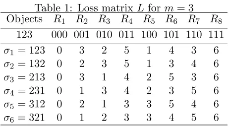
Table 1: Loss matrixL form= 3
Objects R1 R2 R3 R4 R5 R6 R7 R8
123 000 001 010 011 100 101 110 111
σ1 = 123 0 3 2 5 1 4 3 6
σ2 = 132 0 2 3 5 1 3 4 6
σ3 = 213 0 3 1 4 2 5 3 6
σ4 = 231 0 1 3 4 2 3 5 6
σ5 = 312 0 2 1 3 3 5 4 6
σ6 = 321 0 1 2 3 3 4 5 6
Table 2: Feedback matrix H form= 3
Objects R1 R2 R3 R4 R5 R6 R7 R8
123 000 001 010 011 100 101 110 111
σ1 = 123 0 0 0 0 1 1 1 1
σ2 = 132 0 0 0 0 1 1 1 1
σ3 = 213 0 0 1 1 0 0 1 1
σ4 = 231 0 1 0 1 0 1 0 1
σ5 = 312 0 0 1 1 0 0 1 1
σ6 = 321 0 1 0 1 0 1 0 1
of the theory for abstract partial monitoring games developed by Bartok et al. (2014) and Foster and Rakhlin (2012). For ease of understanding, we reproduce the relevant notations and definitions in context of SumLoss. We will specifically mention when we derive results for top k feedback, with general k, and when we restrict to top1 feedback.
Loss and Feedback Matrices: The online learning game with the SumLoss measure and top 1 feedback can be expressed in form of a pair of loss matrix and feedback matrix. The loss matrix L is an m!×2m dimensional matrix, with rows indicating the learner’s actions (permutations) and columns representing adversary’s actions (relevance vectors). The entry in cell (i, j) of L indicates loss suffered when learner plays action i (i.e., σi)
and adversary plays action j (i.e., Rj), that is, Li,j =σi−1·Rj =Pmk=1σ−1i (k)Rj(k). The
feedback matrix H has same dimension asloss matrix, with (i, j) entry being the relevance of top ranked object, i.e.,Hi,j =Rj(σi(1)). When the learner plays actionσi and adversary
plays actionRj, the true loss isLi,j, while the feedback received is Hi,j.
Table 1 and 2 illustrate the matrices, with number of objects m= 3. In both the tables, the permutations indicate rank of each object and relevance vector indicates relevance of each object. For example, σ5 = 312 means object 1 is ranked 3, object 2 is ranked 1 and
object 3 is ranked 2. R5 = 100 means object 1 has relevance level 1 and other two objects
Let `i ∈ R2 m
denote row i of L. Let ∆ be the probability simplex in R2 m
, i.e., ∆ =
{p ∈R2m :∀ 1≤i≤2m, pi ≥0, Ppi = 1}. The following definitions, given for abstract
problems by Bartok et al. (2014), has been refined to fit our problem context.
Definition 1: Learner actioniis called optimal under distributionp∈∆, if`i·p≤`j·p,
for all other learner actions 1≤j≤m!, j 6=i. For every actioni∈[m!], probability cell of
iis defined asCi ={p∈∆ : action iis optimal under p}. If a non-empty cell Ci is 2m−1
dimensional (i.e, elements inCi are defined by only 1 equality constraint), then associated
actioniis called Pareto-optimal.
Note that since entries inH are relevance levels of objects, there can be maximum of 2 distinct elements in each row ofH, i.e., 0 or 1 (assuming binary relevance).
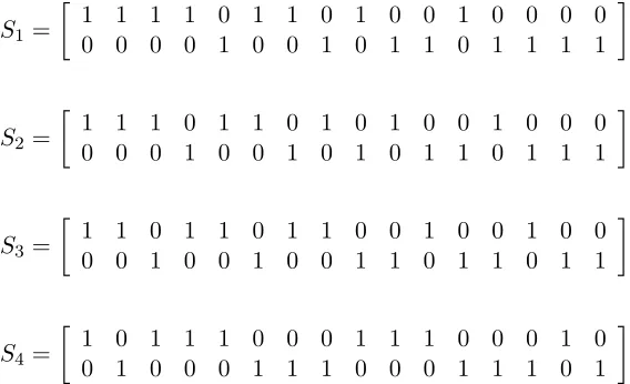
Definition 2: The signal matrix Si, associated with learner’s action σi, is a matrix
with 2 rows and 2m columns, with each entry 0 or 1, i.e., Si ∈ {0,1}2×2 m
. The entries of
`th column of Si are respectively: (Si)1,`=I(Hi,`= 0) and (Si)2,`=I(Hi,` = 1).
Note that by definitions of signal and feedback matrices, the 2nd row of Si (2nd column
ofSi>)) is precisely theith row ofH. The 1st row ofSi (1st column ofSi>)) is the (boolean)
complement ofith row ofH.
2.4 Minimax Regret for SumLoss
The minimax regret for SumLoss, restricted to top 1 feedback, will be established by showing that: a) SumLoss satisfiesglobal observability, and b) it does not satisfy local observability.
2.4.1 Global Observability
Definition 3: The condition of global observability holds, w.r.t. loss matrix L and feed-back matrix H, if for every pair of learner’s actions {σi, σj}, it is true that `i −`j ∈ ⊕k∈[m!]Col(Sk>), whereColrefers to column space (i.e., the vector difference belongs in the column span).
The global observability condition states that the (vector) loss difference between any pair of learner’s actions has to belong to the vector space spanned by columns of (transposed) signal matrices corresponding to all possible learner’s actions. We derive the following theorem on global observability for SumLoss.
Theorem 1. The global observability condition, as per Definition 3, holds w.r.t. loss matrix
L and feedback matrix H defined for SumLoss, for any m≥1.
Proof. For any σa (learner’s action) and Rb (adversary’s action), we have (please see the
end of the proof for explanation of notations and equalities):
La,b=σ−1a ·Rb= m
X
i=1
σa−1(i)Rb(i) 1
=
m
X
j=1
j Rb(σa(j)) 2
=
m
X
j=1
j Rb(˜σj(a)(1)) 3
=
m
X
j=1
j (Sσ>˜j(a))Rb,2.
Thus, we have
`a= [La,1, La,2, . . . , La,2m] =
[
m
X
j=1
j (Sσ>˜j(a))R1,2,
m
X
j=1
j (Sσ>˜j(a))R2,2, ..,
m
X
j=1
j (S˜σ>j(a))R2m,2]
4
=
m
X
j=1
Equality 4 shows that `a is in the column span of m of the m! possible (transposed)
signal matrices, specifically in the span of the 2nd columns of those (transposed) m ma-trices. Hence, for all actions σa, it holds that `a ∈ ⊕k∈[m!]Col(Sk>). This implies that `a−`b ∈ ⊕k∈[m!]Col(Sk>), ∀ σa, σb.
1. Equality 1 holds because σ−1a (i) =j⇒i=σa(j).
2. Equality 2 holds because of the following reason. For any permutation σa and for
every j ∈[m], ∃ a permutation ˜σj(a), s.t. the object which is assigned rank j by σa is the
same object assigned rank 1 by ˜σj(a), i.e., σa(j) = ˜σj(a)(1).
3. In Equality 3, (S> ˜
σj−(1a))Rb,2 indicates theRbth row and 2nd column of (transposed)
sig-nal matrixSσ˜j(a), corresponding to learner action ˜σj(a). Equality 3 holds becauseRb(˜σj(a)(1))
is the entry in the row corresponding to action ˜σj(a) and column corresponding to action Rb of H (see Definition 2).
4. Equality 4 holds from the observation that for a particularj, [(Sσ>˜
j(a))R1,2,(S
> ˜
σj(a))R2,2, . . . ,
(Sσ>˜
j(a))R2m,2] forms the 2nd column of (S
> ˜
σj(a)), i.e., (S
> ˜ σj(a)):,2. 2.4.2 Local Observability
Definition 4: Two Pareto-optimal (learner’s) actionsiandj are calledneighboring actions if Ci ∩Cj is a (2m −2) dimensional polytope (where Ci is probability cell of action σi).
The neighborhood action set of two neighboring (learner’s) actions i and j is defined as
Ni,j+ ={k∈[m!] :Ci∩Cj ⊆Ck}.
Definition 5: A pair of neighboring (learner’s) actions i and j is said to be locally observable if `i−`j ∈ ⊕k∈N+
i,jCol(S >
k). The condition of local observability holds if every
pair of neighboring (learner’s) actions is locally observable.
We now show that local observability condition fails for L, H under SumLoss. First, we present the following two lemmas characterizing Pareto-optimal actions and neighboring actions for SumLoss.
Lemma 2. For SumLoss, each of learner’s action σi is optimal, where
Pareto-optimality has been defined in Definition 1.
Proof. For anyp∈∆, we have`i·p=P2 m j=1 pj (σ
−1
i ·Rj) =σ −1 i ·(
P2m
j=1pjRj) =σ −1 i ·E[R],
where the expectation is taken w.r.t. p. li·pis minimized when ranking of objects according
toσiand expected relevance of objects are in opposite order. That is, the object with highest
expected relevance is ranked 1 and so on. Formally,li·p is minimized whenE[R(σi(1))]≥ E[R(σi(2))]≥. . .≥E[R(σi(m))].
Thus, for actionσi, probability cell is defined asCi={p∈∆ :P2 m
j=1pj = 1, E[R(σi(1))]≥ E[R(σi(2))]≥. . .≥E[R(σi(m))]}. Note that, p∈Ci iff action iis optimal w.r.t. p. Since Ci is obviously non-empty and it has only 1 equality constraint (hence 2m−1 dimensional),
actioniis Pareto optimal.
The above holds true for all learner’s actions σi.
Lemma 3. A pair of learner’s actions {σi, σj} is a neighboring actions pair, if there is
Proof. From Lemma 2, we know that every one of learner’s actions is Pareto-optimal and
Ci, associated with action σi, has structure Ci = {p ∈ ∆ : P2 m
j=1pj = 1, E[R(σi(1))] ≥ E[R(σi(2))]≥. . .≥E[R(σi(m))]}.
Let σi(k) = a, σi(k+ 1) = b. Let it also be true that σj(k) = b, σj(k+ 1) =a and σi(n) =σj(n), ∀n6={k, k+ 1}. Thus, objects in{σi, σj} are same in all places except in
a pair of consecutive places where the objects are interchanged. Then, Ci ∩Cj ={p ∈∆ : P2
m
j=1pj = 1, E[R(σi(1)] ≥ . . . ≥E[R(σi(k)] = E[R(σi(k+
1)] ≥ . . . ≥ E[R(σi(m)]}. Hence, there are two equalities in the non-empty set Ci ∩Cj
and it is an (2m−2) dimensional polytope. Hence condition of Definition 4 holds true and
{σi, σj}are neighboring actions pair.
Lemma 2 and 3 are used to establish the following result:
Theorem 4. The local observability condition, as per Definition 5, fails w.r.t. loss matrix
L and feedback matrix H defined for SumLoss, already at m= 3.
Proof. We will explicitly show that local observability condition fails by considering the case when number of objects is m = 3. Specifically, action pair {σ1, σ2}, in Table 1 are
neighboring actions, using Lemma 3 . Now every other action{σ3, σ4, σ5, σ6} either places
object 2 at top or object 3 at top. It is obvious that the set of probabilities for which
E[R(1)] ≥E[R(2)] =E[R(3)] cannot be a subset of any C3, C4, C5, C6. From Def. 4, the
neighborhood action set of actions {σ1, σ2} is precisely σ1 and σ2 and contains no other
actions. By definition of signal matrices Sσ1, Sσ2 and entries `1, `2 in Table 1 and 2, we
have,
Sσ1 =Sσ2 =
1 1 1 1 0 0 0 0
0 0 0 0 1 1 1 1
`1−`2 =
0 1 −1 0 0 1 −1 0 .
(3)
It is clear that `1−`2∈/ Col(Sσ>1). Hence, Definition 5 fails to hold.
2.5 Minimax Regret Bound
We establish the minimax regret for SumLoss by combining results on global and local observability. First, we get a lower bound by combining our Theorem 4 with Theorem 4 of Bartok et al. (2014).
Corollary 5. Consider the online game for SumLoss with top-1feedback andm= 3. Then, for every learner’s algorithm, there is an adversary strategy generating relevance vectors, such that the expected regret of the learner is Ω(T2/3).
The fact that the game is globally observable ( Theorem 1), combined with Theorem 3.1 in Cesa-Bianchi et al. (2006), gives an algorithm (inspired by the algorithm originally given in Piccolboni and Schindelhauer (2001)) obtainingO(T2/3) regret.
However, the algorithm in Cesa-Bianchi et al. (2006) is intractable in our setting since the algorithm necessarily enumerates all the actions of the learner in each round, which is exponential inmin our case (m! to be exact). Moreover, the regret bound of the algorithm also has a linear dependence on the number of actions, which renders the bound useless.
Discussion: The results above establish that the minimax regret for SumLoss,restricted to top-1feedback, is Θ(T2/3). Theorem 4 of Bartok et al. (2014) says the following: A partial monitoring game which is both globally and locally observable has minimax regret Θ(T1/2), while a game which is globally observable but not locally observable has minimax regret Θ(T2/3). In Theorem 1, we proved global observability, when feedback is restricted to relevance of top ranked item. The global observability result automatically extends to feedback on top k items, for k > 1. This is because for top k feedback, with k > 1, the learner receives strictly greater information at end of each round than top 1 feedback (for example, the learner can just throw away relevance feedback on items ranked 2nd onwards). So, with top k feedback, for general k, the game will remain at least globally observable. In fact, our algorithm in the next section will achieve O(T2/3) regret bound for SumLoss with topk feedback,k≥1. However, the same is not true for failure of local observability. Feedback on more than top ranked item can make the game strictly easier for the learner and may make local observability condition hold, for some k >1. In fact, for k=m (full feedback), the game will be a simple full information game (disregarding computational complexity), and hence locally observable.
2.6 Algorithm for Obtaining Minimax Regret under SumLoss with Top k Feedback
We first provide a general algorithmic framework for getting an O(T2/3) regret bound for SumLoss, with feedback on topk ranked items per round, for k≥1. We then instantiate a specific algorithm, which spends O(mlogm) time per round (thus, highly efficient) and obtains a regret of rate O(poly(m) T2/3).
2.6.1 General Algorithmic Framework
Our algorithm combines blocking with a randomized full information algorithm. We first divide time horizon T into blocks (referred to as blocking). Within each block, we allot a small number of rounds for pure exploration, which allows us to estimate the average of the full relevance vectors generated by the adversary in that block. The estimated average vector is cumulated over blocks and then fed to a full information algorithm for the next block. The randomized full information algorithm exploits the information received at the beginning of the block to maintain distribution over permutations (learner’s actions). In each round in the new block, actions are chosen according to the distribution and presented to the user.
The key property of the randomized full information algorithm is this: the algorithm should have an expected regret rate ofO(C√T), where the regret is the difference between cumulative loss of the algorithm and cumulative loss of best action in hindsight, over T
Our algorithm is motivated by the reduction from bandit-feedback to full feedback
scheme given in Blum and Mansour (2007). However, the reduction cannot be directly
applied to our problem, because we are not in the bandit setting and hence do not know loss of any action. Further, the algorithm of Blum and Mansour (2007) necessarily spends
N rounds per block to try out each of theN available actions — this is impractical in our setting since N =m!.
Algorithm 1 describes our approach. A key aspect is the formation of estimate of average relevance vector of a block (line 16), for which we have the following lemma:
Lemma 7. Let the average of (full) relevance vectors over the time period {1,2, . . . , t} be
denoted asRavg1:t , that is,Ravg1:t =Pt
n=1 Rn
t ∈R
m. Let{i
1, i2, . . . , idm/ke}bedm/kearbitrary
time points, chosen uniformly at random, without replacement, from {1, . . . , t}. At time pointij, onlyk distinct components of relevance vectorRij, i.e.,{Rij(k·(j−1) + 1), Rij(k·
(j −1) + 2), . . . , Rij(k·j)}, become known, ∀j ∈ {1, . . . ,dm/ke} (for j = dm/ke, there
might be less than k components available). Then the vector formed from the m revealed components, i.e. Rˆt= [Rij(k·(j−1) + 1), Rij(k·(j−1) + 2), . . . , Rij(k·j)]{j=1,2,...,dm/ke}
is an unbiased estimator of Ravg1:t .
Proof. We can write ˆRt = Pdm/kej=1 Pk`=1Rij(k·(j −1) +`)ek·(j−1)+`, where ei is the m
dimensional standard basis vector along coordinate j. Then, taking expectation over the randomly chosen time points, we have: Ei1,...,idm/ke( ˆRt) =
Pdm/ke
j=1 Eij[
Pk
`=1Rij(k·(j−1) + `)ek·(j−1)+`] =Pmj=1
Pk
`=1
Pt
n=1
Rn(k·(j−1) +`)ek·(j−1)+`
t =R
avg 1:t .
Suppose we have a full information algorithm whose regret inT rounds is upper bounded by C√T for some constant C and let CI be the maximum loss that the learner can suffer in a round. Note thatCI depends on the loss used and on the range of the relevance scores. We have the following regret bound, obtained from application of Algorithm 1 on SumLoss with topk feedback.
Theorem 8. LetC, CI be the constants defined above. The expected regret under SumLoss,
obtained by applying Algorithm 1, with relevance feedback on top k ranked items per round (k≥1), and the expectation being taken over randomized learner’s actions σt, is
E
" T X
t=1
SumLoss(σt, Rt)
#
−min
σ T
X
t=1
SumLoss(σt, Rt)≤CIdm/keK+C T √
K. (4)
Optimizing over block size K, the final regret bound is:
E
" T X
t=1
SumLoss(σt, Rt)
#
−min
σ T
X
t=1
SumLoss(σt, Rt)≤2(CI)1/3C2/3dm/ke1/3T2/3. (5)
2.6.2 Computationally Efficient Algorithm with FTPL
Algorithm 1 RankingwithTop-kFeedback(RTop-kF)- Non Contextual
1: T = Time horizon,K= No. of (equal sized) blocks, FI= randomized full information algorithm.
2: Time horizon divided into equal sized blocks{B1, . . . , BK}, whereBi={(i−1)(T /K) + 1, . . . , i(T /K)}.
3: Initialize ˆs0=0∈Rm. Initialize any other parameter specific to FI.
4: Fori= 1, . . . , K
5: Selectdm/ketime points{i1, . . . , idm/ke} from blockBi, uniformly at random, without replacement.
6: Divide the mitems intodm/kecells, withkdistinct items in each cell.1 7: Fort∈Bi
8: Ift=ij∈ {i1, . . . , idm/ke} 9: Exploration round:
10: Output any permutationσtwhich places items ofjth cell in topkpositions (in any order).
11: Receive feedback as relevance of topkitems ofσt(i.e., items ofjth cell).
12: Else
13: Exploitation round:
14: Feed ˆsi−1 to the randomized full information algorithm FI and outputσt according to FI.
15: end for
16: Set ˆRi ∈Rm as vector of relevances of themitems collected during exploration rounds.
17: Update ˆsi = ˆsi−1+ ˆRi.
18: end for
Initialization of parameters: In line 3 of the algorithm, the parameter specific to
FTPL is randomization parameter∈R.
Exploitation round: σt, during exploitation, is sampled by FTPL as follows: sample pt∈[0,1/]m from the product of uniform distribution in each dimension. Output
permu-tationσt=M(ˆsi−1+pt) whereM(y) = argmin σ
σ−1·y.
Discussion: The key reason for using FTPL as the full information algorithm is that the structure of our problem allows the permutation σtto be chosen during exploitation round
via a simple sorting operation onmobjects. This leads to an easily implementable algorithm which spends onlyO(mlogm) time per round (sorting is in fact the most expensive step in the algorithm). The reason that the simple sorting operation does the trick is the following: FTPL onlyimplicitly maintains a distribution overm! actions (permutations) at beginning of each round. Instead of having an explicit probability distribution over each action and sampling from it, FTPL mimics sampling from a distribution over actions by randomly perturbing the information vector received so far (say ˆsi−1 in block Bi) and then sorting
the items by perturbed score. The random perturbation puts an implicit weight on each of the m! actions and sorting is basically sampling according to the weights. This is an advantage over general full information algorithms based on exponential weights, which maintain explicit weight on actions and samples from it. We also note that we are using FTPL with uniform distribution over a hypercube as our perturbation distribution. Other choices, such as the Gaussian distribution, can lead to slightly better dependence on the dimension m (see the discussion following the proof of Corollary 9 in the appendix). Our bounds, therefore, do not necessarily yield the optimal dependence onm.
1
We have the following corollary:
Corollary 9. The expected regret of SumLoss, obtained by applying Algorithm 1, with FTPL full information algorithm and feedback on topkranked items at end of each round (k≥1),
and K=O m
1/3T2/3 dm/ke2/3
!
, =O(√1 mK), is:
E
" T X
t=1
SumLoss(σt, Rt)
#
−min
σ T
X
t=1
SumLoss(σt, Rt)≤O(m7/3dm/ke1/3T2/3). (6)
where O(·) hides some numeric constants.
Assuming that dm/ke ∼m/k, the regret rate in Corollary 9 isO m 8/3T2/3
k1/3
!
2.7 Regret Bounds for PairwiseLoss, DCG and Precision@n
PairwiseLoss: As we saw in Eq. 2, the regret of SumLoss is same as regret of PairwiseLoss. Thus, SumLoss in Corollary 9 can be replaced by PairwiseLoss to get exactly same result.
DCG: All the results of SumLoss can be extended to DCG (see Appendix A). Moreover, the results can be extended even for multi-graded relevance vectors. Thus, the minimax regret under DCG,restricted to feedback on top ranked item, even when the adversary can play multi-graded relevance vectors, is Θ(T2/3).
The main differences between SumLoss and DCG are the following. The former is a loss function; the latter is a gain function. Also, for DCG, f(σ) 6=σ−1 (see definition in Sec.2.2 ) and when relevance is multi-graded, DCG cannot be expressed as f(σ)·R, as clear from definition. Nevertheless, DCG can be expressed as f(σ)·g(R), , where g(R) = [gs(R(1)), gs(R(2)), . . . , gs(R(m))], gs(i) = 2i−1 is constructed from univariate, monotonic, scalar valued functions (g(R) =Rfor binary graded relevance vectors). Thus, Algorithm 1 can be applied (with slight variation), with FTPL full information algorithm and top k
feedback, to achieve regret of O(T2/3) 2. The slight variation is that during exploration rounds, when relevance feedback is collected to form the estimator at end of the block, the relevances should be transformed by function gs(·).. The estimate is then constructed in the transformed space and fed to the full information algorithm. In theexploitation round, the selection of σt remains exactly same as in SumLoss, i.e., σt = M(ˆsi−1 +pt) where M(y) = argmin
σ
σ−1·y. This is because argmax
σ
f(σ)·y= argmin
σ
σ−1·y, by definition of
f(σ) in DCG.
Let relevance vectors chosen by adversary haven+ 1 grades, i.e.,R∈ {0,1, . . . , n}m. In
practice,n is almost always less than 5. We have the following corollary:
Corollary 10. The expected regret of DCG, obtained by applying Algorithm 1, with FTPL full information algorithm and feedback on topkranked items at end of each round (k≥1),
2
Note that there is no problem in applying Lemma 7 to DCG. This is because we are trying to estimate
Pt n=1
g(Rn)
and K=O m
1/3T2/3 dm/ke2/3
!
, =O( 1
(2n−1)2√mK), is:
max
σ T
X
t=1
DCG(σt, Rt)−E
" T X
t=1
DCG(σt, Rt)
#
≤O((2n−1)m4/3dm/ke1/3T2/3). (7)
Assuming thatdm/ke ∼m/k, the regret rate in Corollary 10 isO (2
n−1)m5/3T2/3 k1/3
!
.
Precision@n: Since Precision@n=f(σ)·R, the global observability property of SumLoss can be easily extended to it and Algorithm 1 can be applied, with FTPL full information algorithm and top k feedback, to achieve regret of O(T2/3). In the exploitation round, the selection of σt remains exactly same as in SumLoss, i.e., σt = M(ˆsi−1 +pt) where M(y) = argmin
σ
σ−1·y.
However, the local observability property of SumLoss does not extend to Precision@n. The reason is that while f(·) of SumLoss is strictly monotonic, f(·) of Precision@n is monotonic but not strict. Precision@n depends only on the objects in the top n positions of the ranked list, irrespective of the order. A careful review shows that Lemma 3 fails to extend to the case of Precision@n, due to lack of strict monotonicity. Thus, we cannot define the neighboring action set of the Pareto optimal action pairs, and hence cannot prove or disprove local observability.
We have the following corollary:
Corollary 11. The expected regret of Precision@n, obtained by applying Algorithm 1, with FTPL full information algorithm and feedback on top k ranked items at end of each round
(k≥1), and K =O m
1/3T2/3 dm/ke2/3
!
, =O(√1 mK), is:
max
σ T
X
t=1
P recision@n(σt, Rt)−E
" T X
t=1
P recision@n(σt, Rt)
#
≤O(n m1/3dm/ke1/3T2/3).
(8)
Assuming that dm/ke ∼m/k, the regret rate in Corollary 11 is O n m 2/3T2/3 k1/3
!
.
2.8 Non-Existence of Sublinear Regret Bounds for NDCG, AP and AUC
As stated in Sec. 2.2, NDCG, AP and AUC are normalized versions of measures DCG, Precision@nand PairwiseLoss. We have the following lemma for all these normalized rank-ing measures.
Lemma 12. The global observability condition, as per Definition 1, fails for NDCG, AP and AUC, when feedback is restricted to top ranked item.
Theorem 13. There exists an online game, for NDCG with top-1 feedback, such that for every learner’s algorithm, there is an adversary strategy generating relevance vectors, such that the expected regret of the learner is Ω(T). Furthermore, the same lower bound holds if NDCG is replaced by AP or AUC.
3. Online Ranking with Restricted Feedback- Contextual Setting
All proofs not in the main text are in Appendix B.
3.1 Problem Setting and Learning to Rank Algorithm
First, we introduce some additional notations to Section 2.1. In the contextual setting, each query and associated items (documents) are represented jointly as a feature matrix. Each feature matrix, X∈Rm×d, consists of a list ofm documents, each represented as a feature
vector inRd. The feature matrices are considered side-information (context) and represents
varying items, as opposed to the fixed set of items in the first part of our work. Xi:denotes ith row ofX. We assume feature vectors representing documents are bounded byRD in`2
norm. The relevance vectors are same as before.
As per traditional learning to rank setting with query-document matrices, documents are ranked by a ranking function. The prevalent technique is to represent a ranking function as a scoring function and get ranking by sorting scores in descending order. A linear scoring function produces score vector as fw(X) = Xw = sw ∈ Rm, with w ∈ Rd. Here, sw(i)
represents score of ith document (sw points to scoresbeing generated by using parameter
w). We assume that ranking parameter space is bounded in `2 norm, i.e, kwk2 ≤U,∀ w. πs = argsort(s) is the permutation induced by sorting score vector s in descending order.
As a reminder, a permutation π gives a mapping from ranks to documents andπ−1 gives a mapping from documents to ranks.
Performance of ranking functions are judged, based on the rankings obtained from score vectors, by ranking measures like DCG, AP and others. However, the measures themselves are discontinuous in the score vector produced by the ranking function, leading to intractable optimization problems. Thus, most learning to rank methods are based on minimizing surrogate losses, which can be optimized efficiently. A surrogate φ takes in a score vector
s and relevance vector R and produces a real number, i.e., φ :Rm× {0,1, . . . , n}m 7→ R. φ(·,·) is said to be convex if it is convex in its first argument, for any value of the second argument. Ranking surrogates are designed in such a way that the ranking function learnt by optimizing the surrogates has good performance with respect to ranking measures.
Formal problem setting: We formalize the problem as a game being played between a learner and an adversary overT rounds. The learner’s action set is the uncountably infinite set of score vectors in Rm and the adversary’s action set is all possible relevance vectors,
i.e., (n+ 1)m possible vectors. At round t, the adversary generates a list of documents, represented by a matrixXt∈Rm×d, pertaining to a query (the document list is considered
as side information). The learner receivesXt, produces a score vector ˜st∈Rmand ranks the
documents by sorting according to score vector. The adversary then generates a relevance vector Rt but only reveals the relevances of top k ranked documents to the learner. The
As is standard in online learning setting, the learner’s performance is measured in terms of its expected regret:
E
" T X
t=1
φ(˜st, Rt)
#
− min
kwk2≤U
T
X
t=1
φ(Xtw, Rt),
where the expectation is taken w.r.t. to randomization of learner’s strategy andXtw=swt
is the score produced by the linear function parameterized by w.
Algorithm 2 Ranking with Top-k Feedback (RTop-kF)- Contextual
1: Exploration parameterγ ∈(0,12), learning parameter η >0, ranking parameterw1 =0∈Rd
2: For t= 1 to T
3: ReceiveXt (document list pertaining to queryqt)
4: Construct score vector swt
t =Xtwtand get permutation σt= argsort(swtt)
5: Qt(s) = (1−γ)δ(s−swtt) +γUniform([0,1]m) (δ is the Dirac Delta function).
6: Sample ˜st∼Qtand output the ranked list ˜σt= argsort(˜st)
(Effectively3, it means ˜σt is drawn fromPt(σ) = (1−γ)I(σ =σt) +m!γ )
7: Receive relevance feedback on top-k items, i.e., (Rt(˜σt(1)), . . . , Rt(˜σt(k)))
8: Suffer loss φ(˜st, Rt) (Neither loss norRtrevealed to learner)
9: Construct ˜zt, an unbiased estimator of gradient ∇w=wtφ(Xtw, Rt), from top-kfeedback.
10: Updatew=wt−ηz˜t
11: wt+1 = min{1,kwkU2}w (Projection onto Euclidean ball of radiusU).
12: End For
Relation between feedback and structure of surrogates: Algorithm 2 is our general algorithm for learning a ranking function, online, from partial feedback. The key step in Algorithm 2 is the construction of the unbiased estimator ˜ztof the surrogate gradient ∇w=wtφ(Xtw, Rt). The information present for the construction process, at end of round t, is the random score vector ˜st (and associated permutation ˜σt) and relevance of top-k
items of ˜σt, i.e., {Rt(˜σt(1)), . . . , Rt(˜σt(k)}. Let Et[·] be the expectation operator w.r.t. to
randomization at roundt, conditioned on (w1, . . . , wt). Then ˜ztbeing an unbiased estimator
of gradient of surrogate, w.r.twt, means the following: Et[˜zt] =∇w=wtφ(Xtw, Rt). We note
that conditioned on the past, the score vector swt
t =Xtwt is deterministic. We start with
a general result relating feedback to the construction of unbiased estimator of a vector valued function. Let Sm be the set of m! permutations of [m]. Let P denote a probability
distribution on Sm, i.e, Pσ∈SmP(σ) = 1. For a distinct set of indices (j1, j2, . . . , jk) ⊆
[m], we denotep(ji, j2, . . . , jk) as the the sum of probability of permutations whose firstk
objects match objects (j1, . . . , jk), in order. Formally, p(j1, . . . , jk) =
X
π∈Sm
P(π)I(π(1) =j1, . . . , π(k) =jk). (9)
We have the following lemma relating feedback and structure of surrogates:
3 ˜
Lemma 14. Let F : Rm 7→ Ra be a vector valued function, where m ≥ 1, a ≥ 1. For
a fixed x ∈ Rm, let k entries of x be observed at random. That is, for a fixed probability
distribution P and some random σ ∼ P(Sm), observed tuple is {σ, xσ(1), . . . , xσ(k)}. A
necessary condition for existence of an unbiased estimator of F(x), that can be constructed from {σ, xσ(1), . . . , xσ(k)}, is that it should be possible to decompose F(x) over k (or less)
coordinates of x at a time. That is, F(x) should have the structure:
F(x) = X
(i1,i2,...,i`)∈ mP`
hi1,i2,...,i`(xi1, xi2, . . . , xi`) (10)
where `≤k, mP` is ` permutations of m and h:R` 7→Ra (the subscripts in h are used to
denote possibly different functions in the decomposition structure). Moreover, when F(x) can be written in form of Eq 10 , with ` = k, an unbiased estimator of F(x), based on
{σ, xσ(1), . . . , xσ(k)}, is,
g(σ,xσ(1), . . . , xσ(k)) =
P
(j1,j2,...,jk)∈Sk
hσ(j1),...,σ(jk)(xσ(j1), . . . , xσ(jk))
P
(j1,...,jk)∈Sk
p(σ(j1), . . . , σ(jk))
(11)
where Sk is the set ofk! permutations of[k] and p(σ(1), . . . , σ(k))is as in Eq 9 .
Illustrative Examples: We provide simple examples to concretely illustrate the ab-stract functions in Lemma 14. LetF(·) be the identity function, andx∈Rm. Thus,F(x) = x and the function decomposes over k = 1 coordinate of x as follows: F(x) = Pm
i=1xiei,
whereei∈Rm is the standard basis vector along coordinatei. Hence, hi(xi) =xiei. Based
on top-1 feedback, following is an unbiased estimator of F(x): g(σ, xσ(1)) = xσ(1)eσ(1)
p(σ(1)) ,
where p(σ(1)) = P
π∈Sm
P(π)I(π(1) = σ(1)). In another example, let F : R3 7→ R2 and x ∈ R3. Let F(x) = [x1 +x2;x2+x3]>. Then the function decomposes over k= 1
coor-dinate of x as F(x) = x1e1 +x2(e1 +e2) +x3e2, where ei ∈ R2. Hence, h1(x1) = x1e1, h2(x2) =x2(e1+e2) andh3(x3) =x3e2. An unbiased estimator based on top-1 feedback is: g(σ, xσ(1)) =
hσ(1)(xσ(1)) p(σ(1)) .
3.2 Unbiased Estimators of Gradients of Surrogates
Algorithm 2 can be implemented for any ranking surrogate as long as an unbiased estimator of the gradient can be constructed from the random feedback. We will use techniques from online convex optimization to obtain formal regret guarantees. We will thus construct the unbiased estimator of four major ranking surrogates. Three of them are popularconvex surrogates, one each from the three major learning to rank methods, i.e.,pointwise,pairwise and listwise methods. The fourth one is a popularnon-convex surrogate.
Shorthand notations: We note that by chain rule,∇w=wtφ(Xtw, Rt)=X >
t ∇swtt φ(s wt t , Rt),
whereswt
t =Xtwt. SinceXtis deterministic in our setting, we focus on unbiased estimators
of ∇swt t φ(s
wt
in our derivations, we dropw fromsw and the subscripttthroughout. Thus, in our deriva-tions, ˜z = ˜zt,X =Xt, s= swtt (and not ˜st), σ = ˜σt (and not σt), R = Rt, ei is standard
basis vector in Rm along coordinate i and p(·) as in Eq. 9 with P = Pt where Pt is the
distribution in round tin Algorithm 2.
3.2.1 Convex Surrogates
Pointwise Method: We will construct the unbiased estimator of the gradient of squared loss (Cossock and Zhang, 2006): φsq(s, R) =ks−Rk22. The gradient ∇sφsq(s, R) is 2(s−
R) ∈ Rm. As we have already demonstrated in the example following Lemma 14, we
can construct unbiased estimator of R from top-1 feedback ({σ, R(σ(1))}). Concretely, the unbiased estimator is:
˜
z=X>
2
s− R(σ(1))eσ(1) p(σ(1))
.
Pairwise Method: We will construct the unbiased estimator of the gradient of hinge-like surrogate in RankSVM (Joachims, 2002): φsvm(s, R) =
P
i6=j=1I(R(i)> R(j)) max(0,1+ s(j)−s(i)). The gradient is given by:
∇sφsvm(s, R) = m
X
i=1 m
X
j=1,j6=i
I(R(i)> R(j))I(1 +s(j)> s(i))(ej−ei)∈Rm.
Since sis a known quantity, from Lemma 14, we can constructF(R) as follows:
F(R) =Fs(R) = m
X
i=1 m
X
j=1,j6=i
hs,i,j(R(i), R(j)), hs,i,j(R(i), R(j)) =I(R(i)> R(j))I(1+s(j)> s(i))(ej−ei).
SinceFs(R) is decomposable over 2 coordinates ofRat a time,we can construct an unbiased
estimator from top-2 feedback ({σ, R(σ(1)), R(σ(2))}). The unbiased estimator is:
˜
z=X>
h
s,σ(1),σ(2)(R(σ(1)), R(σ(2))) +hs,σ(2),σ(1)(R(σ(2)), R(σ(1))) p(σ(1), σ(2)) +p(σ(2), σ(1))
.
We note that the unbiased estimator was constructed from top-2 feedback. The following lemma, in conjunction with the necessary condition of Lemma 14 shows that it is the minimum information required to construct the unbiased estimator.
Lemma 15. The gradient of RankSVM surrogate, i.e., φsvm(s, R) cannot be decomposed
over 1 coordinate of R at a time.
Listwise Method: Convex surrogates developed for listwise methods of learning to rank are defined over the entire score vector and relevance vector. Gradients of such surro-gates cannot usually be decomposed over coordinates of the relevance vector. We will focus on the cross-entropy surrogate used in the highly cited ListNet (Cao et al., 2007) ranking algorithm and show how a very natural modification to the surrogate makes its gradient estimable in our partial feedback setting.
formally, the surrogate is defined as follows4. Define m maps from Rm to R as: Pj(v) =
exp(v(j))/Pm
j=1exp(v(j)) for j ∈ [m]. Then, for score vector s and relevance vector R, φLN(s, R) =−Pmi=1Pi(R) logPi(s) and∇sφLN(s, R) =Pmi=1
−Pmexp(R(i)) j=1exp(R(j))+
exp(s(i))
Pm
j=1exp(s(j))
ei.
We have the following lemma about the gradient of φLN.
Lemma 16. The gradient of ListNet surrogateφLN(s, R) cannot be decomposed overk, for k= 1,2, coordinates of R at a time.
In fact, an examination of the proof of the above lemma reveals that decomposability at any k < mdoes not hold for the gradient of LisNet surrogate, though we only prove it for k = 1,2 (since feedback for top k items with k >2 does not seem practical). Due to Lemma 14, this means that if we want to run Alg. 2 under top-k feedback, a modification of ListNet is needed. We now make such a modification.
We first note that the cross-entropy surrogate of ListNet can be easily obtained from a standard divergence, viz. Kullback-Liebler divergence. Let p, q ∈ Rm be 2 probability
distributions (Pm i=1pi =
Pm
i=1qi= 1). ThenKL(p, q) =
Pm
i=1pilog(pi)−
Pm
i=1pilog(qi)−
Pm
i=1pi+Pmi=1qi. Takingpi =Pi(R) and qi =Pi(s), ∀ i∈[m] (wherePi(v) is as defined
inφLN) and noting that φLN(s, R) needs to be minimized w.r.t. s (thus we can ignore the
Pm
i=1pilog(pi) term inKL(p, q)), we get the cross entropy surrogate from KL.
Our natural modification now easily follows by considering KL divergence forun-normalized vectors (it should be noted that KL divergence is an instance of a Bregman divergence). Define m maps from Rm to R as: Pj0(v) = exp(v(j)) for j ∈ [m]. Now define pi = Pi0(R)
and qi =Pi0(s). Then, the modified surrogateφKL(s, R) is:
m
X
i=1
eR(i)log(eR(i))− m
X
i=1
eR(i)log(es(i))− m
X
i=1
eR(i)+
m
X
i=1 es(i),
and
m
P
i=1
(exp(s(i))−exp(R(i)))ei is its gradient w.r.t. s. Note that φKL(s, R) is
non-negative and convex in s. Equating gradient to 0 ∈ Rm, at the minimum point, s(i) = R(i), ∀i∈[m]. Thus, the sorted order of optimal score vector agrees with sorted order of relevance vector and it is a valid ranking surrogate.
Now, from Lemma 14, we can constructF(R) as follows: F(R) =Fs(R) =Pmi=1hs,i(R(i)),
where hs,i(R(i)) = (exp(s(i))−exp(R(i)))ei. Since Fs(R) is decomposable over 1
co-ordinate of R at a time, we can construct an unbiased estimator from top-1 feedback
({σ, R(σ(1))}). The unbiased estimator is:
˜ z=X>
(exp(s(σ(1)))−exp(R(σ(1))))e
σ(1) p(σ(1))
Other Listwise Methods: As we mentioned before, most listwise convex surrogates will not be suitable for Algorithm 2 with top-k feedback. For example, the class of popular listwise surrogates that are developed from structured prediction perspective (Chapelle
4
et al., 2007; Yue et al., 2007) cannot have unbiased estimator of gradients from top-k feedback since they are based on maps from full relevance vectors to full rankings and thus cannot be decomposed overk= 1 or 2 coordinates ofR. It does not appear they have any natural modification to make them amenable to our approach.
3.2.2 Non-convex Surrogate
We provide an example of a non-convex surrogate for which Alg. 2 is applicable (however it will not have any regret guarantees due to non-convexity). We choose the SmoothDCG surrogate given in (Chapelle and Wu, 2010), which has been shown to have very com-petitive empirical performance. SmoothDCG, like ListNet, defines a family of surrogates, based on the cut-off point of DCG (see original paper (Chapelle and Wu, 2010) for de-tails). We consider SmoothDCG@1, which is the smooth version of DCG@1 (i.e., DCG which focuses just on the top-ranked document). The surrogate is defined as: φSD(s, R) =
1
Pm
j=1exp(s(j)/)
Pm
i=1G(R(i)) exp(s(i)/), where is a (known) smoothing parameter and G(a) = 2a−1. The gradient of the surrogate is:
[∇sφSD(s, R)] = m
X
i=1
hs,i(R(i)),
hs,i(R(i)) =G(Ri)
m
X
j=1
1
[
exp(s(i)/)
P
j0exp(s(j0)/)
I(i=j)−
exp((s(i) +s(j))/) (P
j0exp(s(j0)/))2 ]ej
Using Lemma 14, we can writeF(R) =Fs(R) =
Pm
i=1hs,i(R(i)) wherehs,i(R(i)) is defined
above. SinceFs(R) is decomposable over 1 coordinate ofR at a time,we can construct an
unbiased estimator from top-1 feedback ({σ, R(σ(1))}), with unbiased estimator being:
s(σ(1))˜z=X>
G(R(σ(1)))
p(σ(1))
m
X
j=1
1
[
exp(s(σ(1))/)
P
j0exp(s(j0)/)
I(σ(1)=j)−
exp((s(σ(1)) +s(j))/) (P
j0exp(s(j0)/))2 ]ej
3.3 Computational Complexity of Algorithm 2
Three of the four key steps governing the complexity of Algorithm 2, i.e., construction of ˜
st, ˜σtand sorting can all be done inO(mlog(m)) time.The only bottleneck could have been
calculations ofp( ˜σt(1)) in squared loss, (modified) ListNet loss and SmoothDCG loss, and p( ˜σt(1),σ˜t(2)) in RankSVM loss, since they involve sum over permutations. However, they
have a compact representation, i.e., p( ˜σt(1)) = (1−γ+ mγ)I( ˜σt(1) =σt(1)) +mγI( ˜σt(1)6= σt(1)) and p( ˜σt(1),σ˜t(2)) = (1−γ + m(m−1)γ )I( ˜σt(1) = σt(1),σ˜t(2) = σt(2)) +m(m−1)γ [∼ I( ˜σt(1) = σt(1),σ˜t(2) = σt(2))]. The calculations follow easily due to the nature of Pt
(step-6 in algorithm) which put equal weights on all permutations other than σt.
3.4 Regret Bounds
The underlying deterministic part of our algorithm is online gradient descent (OGD)
function, as given in Theorem 3.1 of (Flaxman et al., 2005), in our problem setting is:
E
" T X
t=1
φ(Xtwt, Rt)
#
≤ min
w:kwk2≤U
T
X
t=1
φ(Xtw, Rt) + U2
2η + η
2E
" T X
t=1 kz˜tk22
#
(12)
where ˜zt is unbiased estimator of ∇w=wtφ(Xtw, Rt), conditioned on past events, η is the
learning rate and the expectation is taken over all randomness in the algorithm.
However, from the perspective of the loss φ(˜st, Rt) incurred by Algorithm 2, at each
roundt, the RHS above is not a valid upper bound. The algorithms plays the score vector suggested by OGD (˜st=Xtwt) with probability 1−γ (exploitation) and plays a randomly
selected score vector (i.e., a draw from the uniform distribution on [0,1]m), with probability
γ (exploration). Thus, the expected number of rounds in which the algorithm does not follow the score suggested by OGD isγT, leading to an extra regret of order γT. Thus, we have 5
E
" T X
t=1
φ(˜st, Rt)
#
≤E
" T X
t=1
φ(Xtwt, Rt)
#
+O(γT) (13)
We first controlEtkz˜tk22, for all convex surrogates considered in our problem (we remind
that ˜zt is the estimator of a gradient of a surrogate, calculated at time t. In Sec 3.2.1 ,
we omitted showingw insw and index t). To get bound on Etkz˜tk22, we used the following
norm relation that holds for any matrixX(Bhaskara and Vijayaraghavan, 2011): kXkp→q=
sup
v6=0 kXvkq
kvkp , whereqis the dual exponent ofp(i.e., 1 q+
1
p = 1), and the following lemma derived
from it:
Lemma 17. For any 1 ≤ p ≤ ∞, kX>k1→p = kXkq→∞ = maxmj=1kXj:kp, where Xj:
denotes jth row of X and m is the number of rows of matrix.
We have the following result:
Lemma 18. For parameter γ in Algorithm 2 , RD being the bound on `2 norm of the
feature vectors (rows of document matrix X), m being the upper bound on number of doc-uments per query, U being the radius of the Euclidean ball denoting the space of ranking parameters and Rmax being the maximum possible relevance value (in practice always≤5),
letCφ∈ {Csq, Csvm, CKL} be polynomial functions ofR
D, m, U, Rmax, where the degrees of
the polynomials depend on the surrogate (φsq, φsvm, φKL), with no degree ever greater than
four. Then we have,
Etkz˜tk22
≤ C
φ
γ (14)
Plugging Eq. 14 and Eq. 13 in Eq. 12, and optimizing over η and γ, (which gives
η=O(T−2/3) and γ =O(T−1/3)), we get the final regret bound:
5
Theorem 19. For any sequence of instances and labels(Xt, Rt){t∈[T]}, applying Algorithm 2
with top-1 feedback for φsq andφKL and top-2 feedback for φsvm, will produce the following
bound:
E
" T X
t=1
φ(˜st, Rt)
#
− min
w:kwk2≤U
T
X
t=1
φ(Xtw, Rt)≤CφO
T2/3 (15)
where Cφ is a surrogate dependent function, as described in Lemma 18 , and expectation is taken over underlying randomness of the algorithm, over T rounds.
3.5 Impossibility of Sublinear Regret for NDCG Calibrated Surrogates
Learning to rank methods optimize surrogates to learn a ranking function, even though performance is measured by target measures like NDCG. This is done because direct opti-mization of the measures lead to NP-hard optiopti-mization problems. One of the most desirable properties of any surrogate is calibration, i.e., the surrogate should be calibrated w.r.t the target (Bartlett et al., 2006). Intuitively, it means that a function with small expected sur-rogate loss on unseen data should have small expected target loss on unseen data. We focus on NDCG calibrated surrogates (both convex and non-convex) that have been characterized by Ravikumar et al. (2011). We first state the necessary and sufficient condition for a sur-rogate to be calibrated w.r.t NDCG. For any score vectorsand distributionη on relevance space Y, let ¯φ(s, η) = ER∼ηφ(s, R). Moreover, we define G(R) = (G(R1), . . . , G(Rm))>. Z(R) is defined in Sec 2.2.
Theorem 20. (Ravikumar et al., 2011, Thm. 6) A surrogate φis NDCG calibrated iff for any distribution η on relevance space Y, there exists an invertible, order preserving map
g:Rm7→Rm s.t. the unique minimizers∗φ(η) can be written as
s∗φ(η) =g
ER∼η
G(R)
Z(R)
. (16)
Informally, Eq. 16 states that argsort(s∗φ(η))⊆argsort(ER∼η
hG(R)
Z(R)
i
). Ravikumar et al.
(2011) give concrete examples of NDCG calibrated surrogates, including how some of the popular surrogates can be converted into NDCG calibrated ones: e.g., the NDCG calibrated version of squared loss isks−G(Z(R)R)k2
2.
We now state theimpossibility result for the class of NDCG calibrated surrogates when feedback is restricted to top ranked item.
Theorem 21. Fix the online learning to rank game with top 1 feedback and any NDCG calibrated surrogate. Then, for every learner’s algorithm, there exists an adversary strategy such that the learner’s expected regret is Ω(T).
4. Experiments
We conducted experiments on simulated and commercial data sets to demonstrate the performance of our algorithms.
4.1 Non Contextual Setting
Objectives: We had the following objectives while conducting experiments in the non-contextual, online ranking with partial feedback setting:
• Investigate how performance of Algorithm 1 is affected by size of blocks during block-ing.
• Investigate how performance of the algorithm is affected by amount of feedback re-ceived (i.e., generalizingk in topkfeedback).
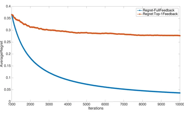
• Demonstrate the difference between regret rate of our algorithm, which operates in partial feedback setting, with regret rate of a full information algorithm which receives full relevance vector feedback at end of each round.
We applied Algorithm 1 in conjunction with Follow-The-Perturbed-Leader (FTPL) full in-formation algorithm, as described in Sec. 2.6. Note that the online learning to rank problem is not as well studied as the batch problem. This is especially true for the partial feedback setting we have. Therefore benchmark data sets with published baseline performance mea-sures, are not available for comparison, to the best of our knowledge. The generic partial monitoring algorithms that do exist cannot be applied due to computational inefficiency (Sec. 2.5).
Experimental Setting: All our experiments were conducted with respect to the DCG measure, which is quite popular in practice, and binary graded relevance vectors. Our ex-periments were conducted on the following simulated data set. We fixed number of items to 20 (m= 20). We then fixed a “true” relevance vector which had 5 items with relevance level 1 and 15 items with relevance level 0. We then created a total of T=10000 relevance vectors by corrupting the true relevance vector. The corrupted copies were created by inde-pendently flipping each relevance level (0 to 1 and vice-versa) with a small probability. The reason for creating adversarial relevance vectors in such a way was to reflect diversity of preferences in practice. In reality, it is likely that most users will have certain similarity in preferences, with small deviations on certain items and certain users. That is, some items are likely to be relevant in general, with most items not relevant to majority of users, with slight deviation from user to user. Moreover, the comparator term in our regret bound (i.e., cumulative loss/gain of the true best ranking in hindsight) makes practical sense if there is a ranking which satisfies most users.
Figure 1: Average regret under DCG, with feedback on top ranked object, for varying block size, where block size isdT /Ke. Best viewed in color.
time horizon T. We wanted to demonstrate how the regret rate (and hence the perfor-mance of the algorithm) differs with different block sizes. The optimal number of blocks in our setting is K ∼ 200, with corresponding block size being dT /Ke = 50. As can be clearly seen, with optimal block size, the regret drops fastest and becomes steady after a point. K = 10 means that block size is 1000. This means over the time horizon, number of exploitation rounds greatly dominates number of exploration rounds, leading to regret dropping at a slower rate initially than than the case with optimal block size. However, the regret drops of pretty sharply later on. This is because the relevance vectors are slightly corrupted copies of a “true” relevance vector and the algorithm gets a good estimate of the true relevance vector quickly and then more exploitation helps. WhenK = 400 (i.e., block size is 25), most of the time, the algorithm is exploring, leading to a substantially worse regret and poor performance.
Figure 2 demonstrates the effect of amount of feedback on the regret rate under DCG. We fixedK = 200, and varied feedback as relevance of topkranked items per round, where
k= 1,5,10. Validating our regret bound, we see that as kincreases, the regret decreases.
Figure 2: Average regret under DCG, where K = 200, for varying amount of feedback. Best viewed in color.