Robust Discriminative Clustering with Sparse Regularizers
Nicolas Flammarion1
Balamurugan Palaniappan2
Francis Bach1 [email protected]
1INRIA
D´epartement d’Informatique de l’ENS, ´Ecole Normale Sup´erieure, CNRS, PSL Research University Paris, France.
2Signal, Statistique et Apprentissage (S2A) Group, IDS Department, LTCI
Telecom-ParisTech Paris, France.
Editor:Sathiya Keerthi
Abstract
Clustering high-dimensional data often requires some form of dimensionality reduction, where clustered variables are separated from “noise-looking” variables. We cast this prob-lem as finding a low-dimensional projection of the data which is well-clustered. This yields a one-dimensional projection in the simplest situation with two clusters, and extends nat-urally to a multi-label scenario for more than two clusters. In this paper, (a) we first show that this joint clustering and dimension reduction formulation is equivalent to pre-viously proposed discriminative clustering frameworks, thus leading to convex relaxations of the problem; (b) we propose a novel sparse extension, which is still cast as a convex relaxation and allows estimation in higher dimensions; (c) we propose a natural extension for the multi-label scenario; (d) we provide a new theoretical analysis of the performance of these formulations with a simple probabilistic model, leading to scalings over the form
d=O(√n) for the affine invariant case and d=O(n) for the sparse case, wheren is the number of examples anddthe ambient dimension; and finally, (e) we propose an efficient iterative algorithm with running-time complexity proportional to O(nd2), improving on earlier algorithms for discriminative clustering with the square loss, which had quadratic complexity in the number of examples.
1. Introduction
Clustering is an important and commonly used pre-processing tool in many machine learn-ing applications, with classical algorithms such as K-means (MacQueen, 1967), linkage algorithms (Gower and Ross, 1969) or spectral clustering (Ng et al., 2002). In high di-mensions, these unsupervised learning algorithms typically have problems identifying the underlying optimal discrete nature of the data; for example, they are quickly perturbed by adding a few noisy dimensions. Clustering high-dimensional data thus requires some form of dimensionality reduction, where clustered variables are separated from non-informative “noise-looking” (e.g., Gaussian) variables.
Several frameworks aim at linearly separating noise from signal, that is finding projec-tions of the data that extracts the signal and removes the noise. They differ in the ways
c
signals and noise are defined. A line of work that dates back to projection pursuit (Friedman and Stuetzle, 1981) and independent component analysis (Hyv¨arinen et al., 2004) defines the noise as Gaussian while the signal is non-Gaussian (Blanchard et al., 2006; Le Roux and Bach, 2013; Diederichs et al., 2013). In this work, we follow De la Torre and Kanade (2006); Ding and Li (2007), along the alternative route where one defines the signal as being clustered while the noise is any non-clustered variable. In the simplest situation with two clusters, we may project the data into a one-dimensional subspace. Given a data matrix
X ∈Rn×dcomposed of n d-dimensional points, the goal is to find a direction w∈Rd such that Xw∈Rn is well-clustered, e.g., byK-means. This is equivalent to identifying both a
direction to project, represented as w ∈ Rd and the labeling y ∈ {−1,1}n that represents
the partition into two clusters.
Most existing formulations are non-convex and typically perform a form of alternating optimization (De la Torre and Kanade, 2006; Ding and Li, 2007), where giveny∈ {−1,1}n,
the projection w is found by linear discriminant analysis (or any binary classification method), and given the projection w, the clustering is obtained by thresholding Xw or runningK-means on Xw. As shown in Section 2, this alternating minimization procedure happens to be equivalent to maximizing the (centered) correlation between y ∈ {−1,1}n
and the projection Xw∈Rd, that is
max
w∈Rd,y∈{−1,1}n
(y>ΠnXw)2
kΠnyk22kΠnXwk22
,
where Πn =In− n11n1>n is the usual centering projection matrix (with 1n∈ Rn being the vector of all ones, and In then×nidentity matrix). This correlation is equal to one when
the projection is perfectly clustered (independently of the number of elements per cluster). Existing methods are alternating minimization algorithms with no theoretical guarantees.
In this paper, we relate this formulation to discriminative clustering formulations (Xu et al., 2004; Bach and Harchaoui, 2007), which consider the problem
min
v∈Rd, b∈R, y∈{−1,1}n 1
nky−Xv−b1nk
2
2, (1)
with the intuition of finding labelsy which are easy to predict by an affine function of the data. In particular, we show that given the relationship between the number of positive labels and negative labels (i.e., the squared difference between the respective number of elements), these two problems are equivalent, and hence discriminative clustering explicitly performs joint dimension reduction and clustering.
When there are more than two clusters, one considers either themulti-labelor the multi-class settings. The multi-class problem assumes that the data are clustered into distinct classes, i.e., a single class per observation, whereas the multi-label problem assumes the data share different labels, i.e., multiple labels per observation. We show in this work that discriminative clustering framework extends more naturally to multi-label scenarios and that this extension has the same convex relaxation.
A summary of the contributions of this paper follows:
− In Section 2, we relate discriminative clustering with the square loss to a joint clus-tering and dimension reduction formulation. The proposed formulation takes care of the balancing hyperparameter implicitly.
− We propose in Section 3, a novel sparse extension to discriminative clustering and show that it can still be cast through a convex relaxation.
− When there are more than two clusters, we extend naturally the sparse formulation to a multi-label scenario in Section 4.
− We then proceed to provide a theoretical analysis of the proposed formulations with a simple probabilistic model in Section 5, which effectively leads to scalings over the form d=O(√n) for the affine invariant case and d=O(n) for the 1-sparse case.
− Finally, we propose in Section 6 efficient iterative algorithms with running-time com-plexity for each step equal toO(nd2), the first to be linear in the number of observa-tionsnfor discriminative clustering with the square loss.
Throughout this paper we assume thatX∈Rn×d iscentered, a common pre-processing
step in unsupervised (and supervised) learning. This implies thatX>1n= 0 and ΠnX=X.
2. Joint Dimension Reduction and Clustering
In this section, we focus on the single binary label case, where we first study the usual non-convex formulation, before deriving non-convex relaxations based on semi-definite programming. Some of the following results are already known in the literature; however, we state them here for completeness.
2.1 Non-convex formulation
Following De la Torre and Kanade (2006); Ding and Li (2007); Ye et al. (2008), we consider a cost function which depends on y∈ {−1,1}n and w∈
Rd, which is such that alternating optimization is exactly (a) runningK-means with two clusters on Xwto obtain y given w
(when we say “running K-means”, we mean solving the vector quantization problem ex-actly), and (b) performing linear discriminant analysis to obtainw given y.
Proposition 1 (Joint clustering and dimension reduction for two clusters) Given
X∈Rn×d such that X>1
n= 0 and X has rank d, consider the optimization problem
max
w∈Rd,y∈{−1,1}n
(y>Xw)2
kΠnyk22kXwk22
Given y, the optimalw is obtained as w= (X>X)−1X>y, while given w, the optimal y is obtained by running K-means onXw.
This equivalence might be straightforward, however it has not been precisely stated in the literature to the best of our knowledge.
Proof Given y, we need to optimize the Rayleigh quotient w>wX>>Xyy>Xw>Xw with a rank-one
matrix in the numerator, which leads to w = (X>X)−1X>y. Given w, we show in Ap-pendix A, that the averaged distortion measure of K-means once the means have been optimized is exactly equal to (y>Xw)2/kΠnyk22.
Algorithm. The proposition above leads to an alternating optimization algorithm. Note that K-means in one dimension may be run exactly in O(nlogn) (Bellman, 1973). After having optimized with respect to w in Eq. (2), we then need to maximize with respect to
y the function y>X(XkΠn>Xy)k−12 X>y 2
, which happens to be exactly performing K-means on the
whitened data (which is now in high dimension and not in 1 dimension). At first, it seems that dimension reduction is simply equivalent to whitening the data and performing K -means; while this is a formally correct statement, the resultingK-means problem is not easy to solve as the clustered dimension is hidden in noise; for example, algorithms such asK -means++ (Arthur and Vassilvitskii, 2007), which have a multiplicative theoretical guarantee on the final distortion measure, are not provably effective here because the minimal final distortion is not small (since the clusters are corrupted by some noisy dimensions), and the multiplicative guarantee is then meaningless.
2.2 Convex relaxation and discriminative clustering
The discriminative clustering formulation in Eq. (1) may be optimized for anyy∈ {−1,1}n
in closed form with respect to basb= 1>n(y−Xv)
n =
1>ny
n sinceX is centered. Substituting b
in Eq. (1) leads us to
min
v∈Rd 1
nkΠny−Xvk
2 2 =
1
nkΠnyk
2
2−max w∈Rd
(y>Xw)2
kXwk2 2
, (3)
wherev is obtained from any solution wasv=wkyXw>Xwk2 2
. Thus, given
(y>1n)2
n2 =
1
n2 #{i, yi= 1} −#{i, yi=−1} 2
=α∈[0,1], (4)
which characterizes the asymmetry between clusters and withkΠnyk2 =n(1−α), we obtain
from Eq. (3), an equivalent formulation to Eq. (2) (with the added constraint) as
min
y∈{−1,1}n, v∈
Rd
1
nkΠny−Xvk
2
2 such that
(y>1n)2
n2 =α. (5)
have formally established that the discriminative clustering formulation in Eq. (5) is related to the joint clustering and dimension reduction formulation in Eq. (2). Following Bach and Harchaoui (2007), we may optimize Eq. (5) in closed form with respect to v as v = (X>X)−1X>y. Substituting v in Eq. (5) leads us to
min
y∈{−1,1}n 1
ny
>
Πn−X(X>X)−1X>
y such that (y
>1 n)2
n2 =α. (6)
This combinatorial optimization problem is NP-hard in general (Karp, 1972; Garey et al., 1976). Hence in practice, it is classical to consider the following convex relaxation of Eq. (6) (Luo et al., 2010). For any admissible y ∈ {−1,+1}n, the matrix Y = yy> ∈
Rn×n is a rank-one symmetric positive semi-definite matrix with unit diagonal entries and conversely any such Y may be written in the form Y = yy> such that y is admissible for Eq. (6). Moreover by rewriting Eq. (6) as
min
y∈{−1,1}n 1
ntryy
>
Πn−X(X>X)−1X>
such that 1
>
n(yy>)1n
n2 =α,
we see that the objective and constraints are linear in the matrix Y =yy> and Eq. (6) is equivalent to
min
Y<0,rank(Y)=1,diag(Y)=1 1
ntrY Πn−X(X
>X)−1X>
such that 1
> nY1n
n2 =α.
Then dropping the non-convex rank constraint leads us to the following classical convex relaxation:
min
Y<0,diag(Y)=1 1
ntrY Πn−X(X
>
X)−1X> such that 1
> nY1n
n2 =α. (7)
This is the standard (unregularized) formulation, which is cast as a semi-definite program. The complexity of interior-point methods isO(n7), but efficient algorithms inO(n2) for such problems have been developed due to the relationship with the max-cut problem (Journ´ee et al., 2010; Wen et al., 2012). We note that convex relaxation techniques are also used for semi-supervised methods (De Bie and Cristianini, 2003).
Given the solutionY, one may traditionally obtain a candidatey∈ {−1,1}nby running
K-means on the largest eigenvector ofY or by sampling (Goemans and Williamson, 1995). In this paper, we show in Section 5 that it may be advantageous to consider the first two eigenvectors.
2.3 Unsuccessful full convex relaxation
The formulation in Eq. (7) imposes an extra parameter α that characterises the cluster imbalance. It is tempting to find a direct relaxation of Eq. (2). It turns out to lead to a trivial relaxation, which we outline below.
When optimizing Eq. (2) with respect to w, we obtain the following optimization prob-lem
max
y∈{−1,1}n
y>X(X>X)−1X>y y>Π
ny
leading to a quasi-convex relaxation as
max
Y<0,diag(Y)=1
trY X(X>X)−1X>
tr ΠnY
,
whose solution is found by solving a sequence of convex problems (Boyd and Vandenberghe, 2004, Section 4.2.5). As shown in Appendix B, this may be exactly reformulated as a single convex problem:
max
M<0,diag(M)=1+1>M1 n2
trM X(X>X)−1X>.
Unfortunately, this relaxation always leads to trivial solutions, and we thus need to consider the relaxation in Eq. (7) for several values of α = 1>nY1n/n2 (and then the non-convex
algorithm can be run from the rounded solution of the convex problem, using Eq. (2) as a final objective). Alternatively, we may solve the following penalized problem for several values ofν >0:
min
Y<0,diag(Y)=1 1
ntrY Πn−X(X
>X)−1X> + ν
n21
>
nY1n. (8)
Forν = 0,Y = 1n1>n is always a trivial solution. As outlined in our theoretical section and
as observed in our experiments, it is sufficient to considerν ∈[0,1].
By convex duality (Borwein and Lewis, 2000, Sec. 4.3), both constrained relaxation in Eq. (7) and penalized relaxation in Eq. (8) are formally equivalent for specific choices of constraint parameter α and penalization parameter ν. We will see in Section 6 that the formulation in Eq. (8) is more suitable for algorithmic design (Bach et al., 2012).
2.4 Equivalent relaxations
Optimizing Eq. (5) with respect to v in closed form as in Section 2.2 is feasible with no regularizer or with a quadratic regularizer. However, if one needs to add more complex regularizers, we need a different relaxation. Therefore, we now propose a new formulation of the discriminative clustering framework. We start from the penalized version of Eq. (5),
min
y∈{−1,1}n, v∈
Rd
1
nkΠny−Xvk
2 2+ν
(y>1n)2
n2 , (9)
which we expand as:
min
y∈{−1,1}n, v∈
Rd
1
ntr Πnyy
>− 2
ntrXvy
>+ 1
ntrX
>Xvv>+ν(y>1n)2
n2 , (10)
and relax as, using Y =yy>,P =yv> and V =vv>,
min
V,P,Y
1
ntr ΠnY−
2
ntrP
>X+1
ntrX
>XV +ν1>nY1n
n2 s.t.
Y P P>V
<0, diag(Y) = 1. (11)
However, we get an interesting behavior when optimizing Eq. (11) with respect to P
and Y also in closed form. For ν = 1, we obtain, as shown in Appendix C.2, the following closed form expressions:
Y = Diag(diag(XV X>))−1/2XV X>Diag(diag(XV X>))−1/2
P = Diag(diag(XV X>))−1/2XV,
leading to the problem:
min
V<0 1− 2
n
n X
i=1 q
(XV X>)ii+
1
ntr(V X
>
X). (12)
The formulation above in Eq. (12) is interesting for several reasons: (a) it is formulated as an optimization problem in V ∈ Rd×d, which will lead to algorithms whose running time will depend on n linearly (see Section 6), (b) it allows for easy adding of regularizers (see Section 3), which may be formulated as convex functions of V = vv>. At first sight this seems to be valid only forν = 1. However we now propose a reformulation which can handle all possibleν ∈[0,1) through a simple data augmentation.
Reformulation for any ν When ν ∈[0,1), we may reformulate the objective function in Eq. (9) as follows:
1
nkΠny−Xvk
2 2+ν
(y>1n)2
n2 =
1
nkΠny−Xv+ν
y>1n
n 1nk
2 2− ν
y>1n
n
2 +ν y
>1 n
n
2
= 1
nky−Xv−(1−ν)
y>1n
n 1nk
2 2+
ν
1−ν (1−ν) y>1n
n
2
= min
b∈R
1
nky−Xv−b1nk
2 2+
ν
1−νb
2, (13)
since n1ky −Xv−b1nk22 + 1−ννb
2 can be optimized in closed form with respect to b as
b = (1− ν)y>n1n. Note that the weighted imbalance ratio (1−ν)y>n1n is made as an optimization variable in Eq. (13). Thus we have the following reformulation
min
v∈Rd, y∈{−1,1}n 1
nkΠny−Xvk
2 2+ν
(y>1n)2
n2
= min
v∈Rd, b∈R, y∈{−1,1}n
1
nky−Xv−b1nk
2 2+
ν
1−νb
2, (14)
3. Regularization
There are several natural possibilities. We consider norms Ω such that Ω(w)2 = Γ(ww>)
for a certain convex function Γ; all norms have that form (Bach et al., 2012, Proposition 5.1). When ν= 1, Eq. (12) then becomes
max
V<0 2
n
n X
i=1 q
(XV X>) ii−
1
ntr(V X
>X)−Γ(V). (15)
The quadratic regularizers Γ(V) = tr ΛV have already been tackled by Bach and Harchaoui (2007). They consider the regularized version of problem in Eq. (3)
min
v∈Rd
1
nkΠny−Xvk
2
2+v>Λv, (16)
optimize in closed form with respect to v as v = (X>X+nΛ)−1X>y. Substituting v in Eq. (16) leads them to
min
Y<0,diag(Y)=1 1
ntrY Πn−X(X
>X+nΛ)−1X
.
In this paper, we propose a novel sparse extension to discriminative clustering framework with the square loss. Specifically we formulate a non-trivial sparse regularizer which is a combination of weighted squared `1-norm and`2-norm. It leads to
Γ(V) = tr[Diag(a)V Diag(a)] +kDiag(c)V Diag(c)k1, (17) such that Γ(vv>) =Pd
i=1a2ivi2+ Pd
i=1ci|vi| 2
. This allows to treat all situations simulta-neously, withν= 1 or with ν ∈[0,1). To be more precise, when ν∈[0,1), we can consider in Eq. (14), a problem of size d+ 1 with a design matrix [X,1n] ∈ Rn×(d+1), a direction of projection vb
∈Rd+1 and different weights for the last variable with a
d+1 = 1−νν and
cd+1= 0.
Note that the sparse regularizers onV introduced in this paper are significantly different when compared to the sparse regularizers on variablev in Eq. (3), for example, considered by Wang et al. (2013). A straightforward sparse regularizer onv in Eq. (3), despite leading to a sparse projection, does not yield natural generalizations of the discriminative clustering framework in terms of theory or algorithms.
In our analysis and experiments for the balanced clusters (when ν = 1), the sparse regularization Γ(·) =λk · k1, forλ∈Rwill often be considered. This is equivalent to setting
a= 0dand c=
√
λ1d in Eq. (17). The problem in Eq. (15) then becomes
max
V<0 2
n
n X
i=1 q
(XV X>) ii−
1
ntr(V X
>X)−λkVk
1. (18)
4. Extension to Multiple Labels
The discussion so far has focussed on two clusters. Yet it is key in practice to tackle more clusters. It is worth noting that the discrete formulations in Eq. (2) and Eq. (5) extend directly to more than two clusters. However two different extensions of the initial problems Eq. (2) or Eq. (5) are conceivable. They lead to problems with different constraints on different optimization domains and, consequently, to different relaxations. We discuss these possibilities next.
One extension is the multi-class case. The multi-class problem which is dealt with by Bach and Harchaoui (2007) assumes that the data are clustered into K classes and the various partitions of the data points into clusters are represented by the K-class indicator matricesy ∈ {0,1}n×Ksuch thaty1
K = 1n. The constrainty1K= 1nensures that one data
point belongs to only one cluster. However as discussed by Bach and Harchaoui (2007), by lettingY =yy>, it is possible to lift theseK-class indicator matrices into the outer convex approximationsCK ={Y ∈Rn×n:Y =Y>,diag(Y) = 1
n, Y <0, Y 4 K11n1>n}(Frieze and
Jerrum, 1995), which is different for all values of K. Note that letting K = 2 corresponds to the previous sections.
In this paper, we consider a different novel extension for discriminative clustering to the multi-label case. The multi-label problem assumes that the data share k labels and the data-label membership is represented by matrices y ∈ {−1,+1}n×k. In other words,
the multi-class problem embeds the data in the extreme points of a simplex, while the multi-label problem does so in the extreme points of the hypercube.
The discriminative clustering formulation of the multi-label problem is
min
v∈Rd×k, y∈{−1,1}n×k 1
nkΠny−Xvk
2
F, (19)
where the Frobenius norm is defined for any vector or rectangular matrix as kAk2 F =
trAA> = trA>A. Letting k = 1 here corresponds to the previous sections. The dis-crete ensemble of matricesy∈ {−1,+1}n×k can be naturally lifted intoD
k={Y ∈Rn×n:
Y = Y>,diag(Y) = k1n, Y < 0}, since diag(Y) = diag(yy>) = Pk
i=1yi,i2 = k. As the
optimization problems in Eq. (7) and Eq. (8) have linear objective functions, we can change the variable from Y to ˜Y =Y /k to change the constraint diag(Y) = k1n to diag( ˜Y) = 1n
without changing the optimizer of the problem. Thus the problems can be solved over the relaxed domain D = {Y ∈ Rn×n : Y = Y>,diag(Y) = 1
n, Y < 0} which is independent
of k.
Note that the domain D is similar to that considered in the problems in Eq. (8) and Eq. (11) and these convex relaxations are the same regardless of the value of k. Hence the multi-label problem is a more natural extension of the discriminative framework, with a slight change in how the labels y are recovered from the solution Y (we discuss this in Section 5.3).
5. Theoretical Analysis
is considered first and analysis is provided for both balanced and imbalanced clusters. Our study for the sparse case currently only provides results for the simple 1-sparse solution. However, the analysis also yields valuable insights on the scaling betweennandd. We then derive results for multi-label situation.
For ease of analysis, we consider the constrained problem in Eq. (7), the penalized prob-lem in Eq. (8) or their equivalent relaxations in Eq. (12) or Eq. (18) under various scenarios, for which we use the same proof technique. We first try to characterize the low-rank solu-tions of these relaxasolu-tions and then show in certain simple situasolu-tions the uniqueness of such solutions, which are then non-ambiguously found by convex optimization. Perturbation arguments could extend these results by weakening our assumptions but are not within the scope of this paper, and hence we do not investigate them further in this section.
5.1 Analysis for two clusters: non-sparse problems
In this section, we consider several noise models for the problem, either adding irrelevant dimensions or perturbing the label vector with noise. We consider these separately for simplicity, but they could also be combined (with little extra insight).
5.1.1 Irrelevant dimensions
We consider an “ideal” design matrix X ∈Rn×d such that there exists a direction v along
which the projectionXvis perfectly clustered into two distinct real valuesc1 and c2. Since Eq. (2) is invariant by affine transformation, we can rotate the design matrix X to have
X = [y, Z] with y ∈ {−1,1}n, which is clustered into +1 or −1 along the direction v = 1
0d−1
. Then after being centered, the design matrix is written as X = [Πny, Z] with
Z = [z1, . . . , zd−1]∈Rn×(d−1). The columns ofZ represent the noisy irrelevant dimensions
added on top of the signaly.
5.1.2 Balanced problem
When the problem is well balanced (y>1n= 0), y is already centered and Πny =y. Thus
the design matrix is represented asX = [y, Z]. We consider here the penalized formulation in Eq. (8) with ν= 1 which is the only scenario where we are able to provide a theoretical analysis.
Let us assume that the columns (zi)i=1,...,d−1ofZare i.i.d. with symmetric distributionz, withEz=Ez3= 0 and such that kzk∞ is almost surely bounded by R≥0. We denote by
Ez2 =m its second moment and byEz4/(Ez2)2 =β its (unnormalized) kurtosis.
Surprisingly the clustered vector yhappens to generate a solutionyy> of the relaxation Eq. (8) for all possible values ofZ (see Lemma 11 in Appendix D.2 ). However the problem in Eq. (8) should have aunique solution in order to always recover the correct assignment
y. Unfortunately the semidefinite constraint Y < 0 of the relaxation makes the second-order information arduous to study. Due to this reason, we consider the other equivalent relaxation in Eq. (12) for which V∗ = vv> is also solution with v ∝ (X>X)−1X>y (see
already provides unicity for the unconstrained problem. Hence we are able to ensure the uniqueness of the solution with high probability.
Proposition 2 Let us assume d≥3, β >1 andm2≥ 2(dβ+−β3−4):
(a) If n ≥ d2R4 1+(m2d(+ββ−)1)m2, V∗ is the unique solution of the problem in Eq. (12) with high
probability.
(b) If n≥ min{m2(βd−2R1)4,2m2,2m}, v is the principal eigenvector of any solution of the problem
in Eq. (12) with high probability.
Let us make the following observations:
− Proof technique: The proof relies on a computation of the Hessian of f(V) = 2
n Pn
i=1 p
(XV X>)ii−n1 trX>XV which is the objective function in Eq. (12). We
first derive the expectation of ∇2f(V) with respect to the distribution of X. By the law of large numbers, it amounts to havengoing to infinity in∇2f(V). Then we expand the spectrum of this operatorE∇2f(V) to lower-bound its smallest eigenvalue. Finally we use concentration theory on matrices, following Tropp (2012), to bound the Hessian ∇2f(V) for finite n.
− Effect of kurtosis: We remind that β >1, with equality if and only if z follows a Rademacher law (P(z = +1) =P(z=−1) = 1/2). Thus, if the noisy dimensions are clustered, then unsurprisingly, our guarantee is meaningless. Note that the constantβ
behaves like a distance of the distributionzto the Rademacher distribution. Moreover,
β = 3 ifz follows a standard normal distribution.
− Scaling betweendandn: If the noisy variables are not evenly clustered between the same clusters{±1}(i.e.,β >1), we recover a rank-one solution as long as n=O(d3); while, as long as n= O(d2), the solution is not unique but its principal eigenvector recovers the correct clustering. Moreover, as explained in the proof, its spectrum would be very spiky.
− The assumption m2 ≥ 2(dβ+−β3−4) is generally satisfied for large dimensions. Note that
m2dis the total variance of the irrelevant dimensions, and when it is small, i.e., when
m2 ≤ 2(dβ+−β3−4), the problem is particularly simple, and we can also show that V∗ is
the unique solution of the problem in Eq. (12) with high probability if n ≥ d2R4 m2 .
Finally, note that for sub-Gaussian distributions (where β ≤3), the extra constraint is vacuous, while for super-Gaussian distributions (whereβ ≥3), this extra constraint only appears for smallm.
5.1.3 Noise robustness for the one dimensional balanced problem
We assume now that the data are one-dimensional and are perturbed by some noiseε∈Rn
such that X =y+εwith y∈ {−1,1}n. The solution of the relaxation in Eq. (8) recovers
the correcty in this setting only when each component of y and y+ε have the same sign (this is shown in Appendix D.5). This result comes out naturally from the information on whether the signs of y and y+ε are the same or not. Further if we assume that y and ε
are independent, this condition is equivalent to kεk∞<1 almost surely.
5.1.4 Unbalanced problem
When the clusters are imbalanced (y>1n 6= 0), the natural rank-one candidates Y∗ =yy>
andV∗ =vv> are no longer solutions of the relaxations in Eq. (8) (forν = 1) and Eq. (12),
as proved in Appendix D.6. Nevertheless we are able to characterize some solutions of the penalized relaxation in Eq. (8) forν = 0.
Lemma 3 For ν = 0 and for any non-negative a, b∈R such thata+b= 1,
Y =ayy>+b1n1>n
is solution of the penalized relaxation in Eq. (8).
Hence any eigenvector of this solution Y would be supported by the directions y and 1n.
Moreover when the valueα∗ = (1 >
ny
n )2 is known, it turns out that we can characterize some
solutions of the constrained relaxation in Eq. (7), as stated in the following lemma.
Lemma 4 For α≥α∗,
Y = 1−α
1−α∗
yy>+
1− 1−α
1−α∗
1n1>n
is a rank-2 solution of the constrained relaxation in Eq. (7) with constraint parameter α.
The eigenvectors of Y enable to recover y for α∗ ≤ α < 1. We conjecture (and checked
empirically) that this rank-2 solution is unique under similar regimes to those considered for the balanced case. The proof would be more involved since, whenν6= 1, we are not able to derive an equivalent problem inV for the penalized relaxation in Eq. (8) similar to Eq. (12) for the balanced case. We also note that Lemmas 3 and 4 will be direct consequences of Lemma 8 in Section 5.3.
ThusY being rank-2, one should really be careful and consider the first two eigenvectors when recoveringyfrom a solutionY. This can be done by rounding the principal eigenvector of ΠnYΠn= 11−−αα∗Πny(Πny)
> as discussed in the following lemma.
Lemma 5 Let yev be the principal eigenvector of ΠnYΠn where Y is defined in Lemma 4, then
sign(yev) =y.
Proof By definition of Y, yev = q
1−α
1−α∗Πny thus sign(yev) = sign(Πny) and sinceα ≤1
then sign(Πny) = sign(y−
√
In practice, contrary to the standard procedure, we should, for any ν, solve the penalized relaxation in Eq. (8) and then do K-means on the principal eigenvector of the centered solution ΠnYΠn instead of the solution Y to recover the correct y. This procedure is
followed in our experiments on real-world data in Section 7.2.
5.2 Analysis for two clusters: one-sparse problems
We assume here that the direction of projectionv(such thatXv=y) isl-sparse (byl-sparse we mean kvk0 = l). The `1-norm regularized problem in Eq. (18) is no longer invariant by affine transformation and we cannot consider thatX = [y, Z] without loss of generality. Yet the relaxation Eq. (18) seems experimentally to only have rank-one solutions for the simplel = 1 situation. Hence we are able to derive some theoretical analysis only for this case. It is worth noting the l = 1 case is simple since it can be solved in O(d) by using
K-means separately on all dimensions and ranking them. Nonetheless the proposed scaling also holds in practice for l>1 (see Figure 1b).
Thereby we consider data X = [y, Z] with y ∈ {−1,1}n and Z ∈
Rn×(d−1) which are clustered in the direction v = [1,0, . . . ,0]> ∈ Rd. When adding a `
1-penalty, the initial problem in Eq. (5) for α= 0 is
min
y∈{−1,1}n, v∈
Rd
1
nky−Xvk
2
2+λkvk21. (20)
When optimizing in v this problem is close to the Lasso (Tibshirani, 1996) and a solution is known to be vi∗ = (y>y+nλ)−1y>y = 1+1λ, ∀i∈ J and vi∗ = 0, ∀i∈ {1,2, . . . , d} \J ,
whereJ is the support ofv∗. The candidateV∗ =v∗v∗> is still a solution of the relaxation
in Eq. (18) (see Lemma 15 in Appendix E.1) and we will investigate under which conditions on X this solution is unique. Let us assume as before (zi)i=1,...,d are i.i.d. with distribution
z symmetric with Ez =Ez3 = 0, and denote by Ez2 =m and Ez4/(Ez2)2 = β. We also assume that kzk∞ is almost surely bounded by 0 ≤ R ≤ 1. We are able to ensure the
uniqueness of the solution with high-probability.
Proposition 6 Let us assume d≥3.
(a) If n ≥ dR2 1+(m2d(+ββ−)1)m2, V∗ is the unique solution of the problem Eq. (12) with high
probability.
(b) If n≥ m2dR(β2−1), v
∗ is the principal eigenvector of any solution of the problem Eq. (12)
with high probability.
The proof technique is very similar to the one of Proposition 2. With the function
g(V) = n2Pn
i=1 p
(XV X>)
ii−λkVk1 − n1trX>XV, we can certify that g will decrease around the solution V∗ by analyzing the eigenvalues of its Hessian.
The rank-one solution V∗ is recovered by the principal eigenvector of the solution of
the relaxation Eq. (18) as long as n = O(d). Thus we have a much better scaling when compared to the non-sparse setting wheren=O(d2). We also conjecture a scaling of order
5.3 Analysis for the multi-label extension
In this section, the signals share k labels which are corrupted by some extra noisy dimen-sions. We assume the centered design matrix to be X = [Πny, Z] where y ∈ {−1,+1}n×k
and Z ∈Rn×(d−k). We also assume that y is full-rank1. We denote byy= [y
1, . . . , yk] and
αi =
y>
i 1n n
2
fori= 1,· · · , k. We consider the discrete constrained problem
min
v∈Rd×k, y∈{−1,1}n×k 1
nkΠny−Xvk
2
F such that
1>nyy>1n
n2 =α
2, (21)
and the discrete penalized problem forν = 0
min
v∈Rd×k, y∈{−1,1}n×k 1
nkΠny−Xvk
2
F. (22)
As explained in Section 4, these two discrete problems admit the same relaxations in Eq. (7) and Eq. (8) we have studied for one label. We now investigate when the solution of the problems in Eq. (21) and in Eq. (22) generate solutions of the relaxations in Eq. (7) and Eq. (8).
By analogy with Lemma 3, we want to characterize the solutions of these relaxations which are supported by the constant vector 1n and the labels (y1, . . . , yk). Their general
form is Y = ˜yAy˜> where A ∈ Rk×k is symmetric semi-definite positive and ˜y = [1 n, y].
However the initial y is easily recovered from the solution Y only whenA is diagonal. To that end the following lemma derives some condition under which the only matrix A such that the corresponding Y satisfies the constraint of the relaxations in Eq. (7) and Eq. (8) is diagonal.
Lemma 7 The solutions of the matrix equation diag(˜yAy˜>) = 1nwith unknown variable A are diagonal if and only if the family{1n,(yi)1≤i≤k,(yiyj)1≤i<j≤k}is linearly independent where we denoted by the Hadamard (i.e., pointwise) product between matrices.
In this way we are able to characterize the solution of relaxations in Eq. (7) and Eq. (8) with the following result:
Lemma 8 Let us assume that the family {1n,(yi)1≤i≤k,(yiyj)1≤i<j≤k} is linearly inde-pendent. Ifα≥αmin= min
1≤i≤k{αi}with(αi)1≤i≤kdefined above Eq. (21), the solutions of the constrained relaxation in Eq. (7) supported by the vectors (1n, y1,· · · , yk) are of the form:
Y =a201n1>n + k X
i=1
a2iyiy>i ,
where (ai)0≤i≤k satisfies Pk
i=0a2i = 1 and a20+ Pk
i=1a2iαi =α.
Moreover the solutions of the penalized relaxation in Eq. (8) for ν = 0 which are sup-ported by the vectors (1n, y1,· · · , yk) are of the form:
Y =a201n1>n + k X
i=1
a2iyiy>i ,
where (ai)0≤i≤k satisfiesPki=0a2i = 1.
In the multi-label case, some combinations of the constant matrix 1n1>n and the
rank-one matricesyiy>i are solutions of constrained or penalized relaxations. Furthermore, under
some assumptions on the labels (yi)1≤i≤k, these combinations are the only solutions which
are supported by the vectors (1n, y1,· · · , yk). And we conjecture (and checked empirically)
that under assumptions similar to those made for the balanced one-label case, all the solu-tions of the relaxation are supported by the family (1n, y1,· · · , yk) and consequently share
the same form as in Lemma 8. Thus the eigenvector of the solutionY would be in the span of the directions (1n, y1,· · · , yk).
Let us consider an eigenvalue decomposition of Y =F F>=Pk
i=0λieie>i and denote by
M = [a01n, a1y1,· · · , akyk] where (ai)0≤i≤k are defined in Lemma 8. Since M M> =F F>,
there is an orthogonal transformation R such that F R=M. We also denote the product
F R by F R = [ξ0,· · ·, ξK]. We propose now an alternating minimization procedure to
recover the labels (y1,· · ·, yk) from M.
Lemma 9 Consider the optimization problem
min
M∈M, R∈Rk×k:R>R=I
k
kF R−Mk2 F,
where M={[a01n, a1y1,· · · , akyk], a∈Rk+1 :kak2 = 1, yi ∈ {±1}n}.
Given M, the problem is equivalent to the orthogonal Procrustes problem (Sch¨onemann, 1966). Denote by U∆V> a singular value decomposition of F>M. The optimal R is obtained as R=U V>. While givenR, the optimal M is obtained as
M = p 1
kξ1k21+kξ2k21+. . .+kξkk21
[kξ0k1sign(ξ0),· · · ,kξkk1sign(ξk)].
Proof We give only the argument for the optimization problem with respect toM. Given
R, the optimization problem inM is equivalent to max
a∈Rk+1:kak
2=1, y∈{−1,1}n×k
tr(F R)>M and
tr(F R)>M =a0ξ0>1n+Pki=1aiξi>yi . Thus by property of the dual norms the solution is
given byyi = sign(ξi) and ai=
kξik1
√
kξ1k2
1+kξ2k21+...+kξkk21
.
The minimization problem in Lemma 9 is non-convex; however we observe that performing few alternating optimizations is sufficient to recover the correct (y1, . . . , yk) fromM. 5.4 Discussion
non-convex problem. Unfortunately the solutions lose the characterized rank when the initial problem is slightly perturbed since the rank of a matrix is not a continuous function. Nevertheless, the spectrum of the new solution is really spiked, and thus these results are quite conservative. We empirically observe that the principal eigenvectors keep recovering the correct information outside these scenarios. However this simple proof mechanism is not easily adaptable to handle perturbed problems in a straightforward way since it is difficult to characterize the properties of eigenvectors of the solution of a semi-definite program. Hence we are able to derive a proper theoretical study only for these simple models.
6. Algorithms
In this section, we present an optimization algorithm which is adapted to largen settings, and avoids the n-dimensional semidefinite constraint.
6.1 Reformulation
We aim to solve the general regularized problem which corresponds to Eq. (15)
max
V<0 2
n
n X
i=1 q
(XV X>) ii−
1
ntrV(X
>X+nDiag(a)2)− kDiag(c)V Diag(c)k
1. (23) We consider a slightly different optimization problem:
max
V<0 1
n
n X
i=1 q
(XV X>)
ii− kDiag(c)V Diag(c)k1 s.t. trV( 1
nX
>X+ Diag(a)2) = 1. (24)
When c is equal to zero, then Eq. (24) is exactly equivalent to Eq. (23); when c is small (as will typically be the case in our experiments), the solutions are very similar—in fact, one can show by Lagrangian duality that by a sequence of problems in Eq. (24), one may obtain the solution to Eq. (23).
6.2 Smoothing
By lettingA=X>nX+Diag(a)2, we consider a strongly-convex approximation of Eq. (24) as:
max
V<0 1
n
n X
i=1 q
(XV X>)ii− kDiag(c)V Diag(c)k1−εtr[(A
1 2V A
1
2) log(A 1 2V A
1 2)]
s.t. tr(A12V A 1
2) = 1, (25)
where −trMlog(M) is a spectral convex function called the von-Neumann entropy (von Neumann, 1927). The difference in the two problems is known to be εlog(d) (Nesterov, 2007). As shown in Appendix G.1, the dual problem is
min
u∈Rn
+,C∈Rd×d:|Cij|6cicj 1 2n
n X
i=1 1
ui
+φε A−12 1
2nX
>Diag(u)X−C
A−12, (26)
6.3 Optimization algorithm
In order to solve Eq. (26), we split the objective function into a smooth part F(u, C) =
φε A−12 1
2nX
>Diag(u)X−C
A−12and a non-smooth partH(u, C) =I|C
ij|6cicj+ 1 2n
Pn i=1u1i. We may then apply FISTA (Beck and Teboulle, 2009) updates to the smooth function
φε(A−12( 1
2nX
>Diag(u)X−C)A−12), along with a proximal operator for the non-smooth
terms I|Cij|6cicj and 1 2n
Pn
i=1u1i, which may be computed efficiently. See details in Ap-pendix G.2.
Running-time complexity. Since we need to project on the SDP cone of size d at each iteration, the running-time complexity per iteration is O(d3+d2n); given that often
n > d, the dominating term is O(d2n). It is still an open problem to make this linear in d. Our function being O(1/ε)-smooth, the convergence rate is of the form O(1/(εt2)). Since we stop when the duality gap is εlog(d) (as we use smoothing, it is not useful to go lower), the number of iterations is of order 1/(εplog(d)). The proposed algorithm is a clear improvement over the existing approach by Bach and Harchaoui (2007) which is quadratic inn.
7. Experiments
We implemented the proposed algorithm in Matlab. The code has been made available in
https://drive.google.com/uc?export=download&id=0B5Bx9jrp7celMk5pOFI4UGt0ZEk. Two sets of experiments were performed: one on synthetically generated data sets and the other on real-world data sets. The details about experiments follow.
7.1 Experiments on synthetic data
In this section, we illustrate our theoretical results and algorithms on synthetic examples. The synthetic data were generated by assuming a fixed clustering with α∗ ∈[0,1], along a
single direction and the remaining variables were whitened. We consider clustering error defined for a predictor ¯y as 1−(¯y>y/n)2, with values in [0,1] and equal to zero if and only ify= ¯y.
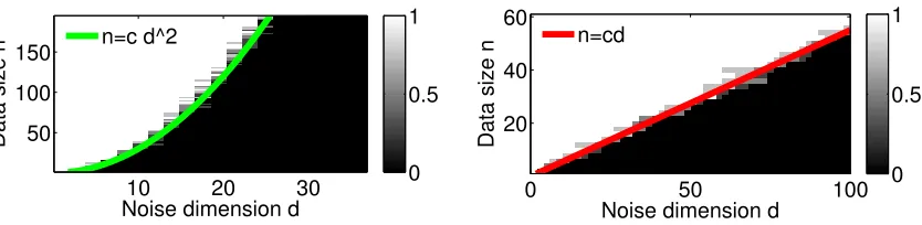
Phase transition. We first illustrate our theoretical results for the balanced case in Figure 1. We solve the relaxation in Eq. (12) and Eq. (18) for a large range of d and n
using the cvx solver (Grant and Boyd, 2008, 2014). We show the results averaged over 4 replications and take λ = 1/√n for the sparse problems. In Figure 1a, we investigate whether cvx finds a rank-one solution for a problem of size (n, d) (the value is 1 if the solution is rank-one and 0 otherwise). We compare the performance of the algorithms without `1-regularization in the affine invariant case and with `1-regularization in the 1-sparse case. We observe a phase transition with a scaling over the form n=O(d2) for the affine invariant case andn=O(d) for the 1-sparse case. This is better than what is expected by the theory and corresponds rather to the performance of the principal eigenvector of the solution. It is worth noting that it may be uncertain to really distinguish between a rank-one solution and a spiked solution.
(without `1-regularization) which corresponds to the affine invariant case, against the `1 -regularized formulation in Eq. (18). We notice a phase transition of the clustering error with a scaling over the formn=O(d2) for the affine invariant case andn=O(d) for the 4-sparse case. It supports our conjecture on the scaling of order n = O(ld) for l-sparse problems. Comparing left plots of Figure 1a and Figure 1b, we observe that the two phase-transitions occur at the same scaling between n and d. Thus there are few values of (n, d) for which the cvx solver finds a solution whose rank is strictly larger than one and whose principal eigenvector has a low clustering error. This illustrates, in practice, this solver aims to find a rank-one solution under the improved scalingn=O(d2).
Noise dimension d
Data size n
10 20 30
50 100 150
0 0.5 1 n=c d^2
Noise dimension d
Data size n
0 50 100
20 40 60
0 0.5 1 n=cd
(a) Phase transition for rank-one solution. Left: affine invariant case. Right: 1-sparse case.
Noise dimension d
Data size n
10 20 30 40 50 100
200 300 400
0 0.5 1 n=c d2
Noise dimension d
Data size n
10 20 30 40 50 100
200 300 400
0 0.5 1 n=c d
(b) Phase transition for clustering error. Left: affine invariant case . Right: 4-sparse case.
Figure 1: Phase transition plots.
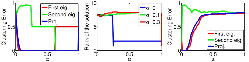
Unbalanced case. We generate an unbalanced problem ford= 10,n= 80 andα∗ = 0.25
0 0.5 1 0
0.5 1
α
Clustering Error
First eig. Second eig. Proj.
0 0.5 1
0 5 10
α
Rank of the solution
σ=0
σ=0.1
σ=0.3
0 0.5 1
0 0.5 1
µ
Clustering Error
First eig. Second eig. Proj.
Figure 2: Unbalanced problem for n= 80, d= 10 and α∗ = 0.25. Left: Clustering error
for the constrained relaxation. Middle: Rank of the solution for different level of noise σ. Right: Clustering error for the penalized relaxation.
recovered for ν close to 0 by the first eigenvector and the projection method whereas the second one performs always badly. (c) When there is zero noise the rank of the solution is one for α∈ {α∗,1}, two for α ∈(α∗,1) and greater otherwise. These findings confirm our
analysis. However, wheny is corrupted by some noise this result is no longer true.
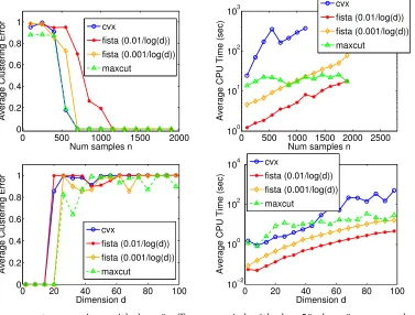
Runtime experiments. We generated data with ak-sparse direction of projection v by adding d−k noise variables to a randomly generated and rotated k-dimension data. The scalability of the FISTA based optimization algorithm illustrated in Section 6.3 to solve Eq. (24) (with c = √λ1d, a = 0d) was compared against a benchmark cvx solver (which
solves Eq. (18)). Experiments were performed for λ = 0 and λ = 0.001, the coefficient associated with the sparse kVk1 term. For a fixed d, cvx breaks down for large n values (typicallyn>1000). Similarly, the runtime required by cvxis generally high forλ= 0 and is comparable to our method forλ= 0.001. This behavior is illustrated in Figure 3.
When λ = 0, the problem reduces exactly to the original Diffrac problem (Bach and Harchaoui, 2007). In the plots in Figure 3a our implementation using FISTA is compared to the baseline Diffrac which is solved with max-cut SDP (Boumal et al., 2014). We observed that our method is comparable in terms of runtime and clustering performance of low-rank methods for max-cut. However, forλ >0, the equivalence with max-cut disappears.
The plots in these figures show the behavior of FISTA for two different stopping criteria:
ε= 10−2/log(d) and ε= 10−3/log(d). It is observed that the choice 10−3/log(d) gives a better accurate solution at the cost of more number of iterations (and hence higher runtime). For sparse problems in Figure 3b, we see that cvx gets a better clustering performance (while crashing for largen); the difference would be reduced with a smaller duality gap for FISTA.
Clustering performance. Experiments comparing the proposed method (Eq. (24) with
c = √λ1d and a = 0d solved using FISTA based optimization algorithm, and Eq. (18)
0 500 1000 1500 2000 0
0.2 0.4 0.6 0.8 1
Num samples n
Average Clustering Error
cvx
fista (0.01/log(d)) fista (0.001/log(d)) maxcut
0 500 1000 1500 2000 2500
100
101
102
103
Num samples n
Average CPU Time (sec)
cvx
fista (0.01/log(d)) fista (0.001/log(d)) maxcut
0 20 40 60 80 100
0 0.2 0.4 0.6 0.8 1
Dimension d
Average Clustering Error
cvx
fista (0.01/log(d)) fista (0.001/log(d)) maxcut
0 20 40 60 80 100
10−2
100
102
104
Dimension d
Average CPU Time (sec)
cvx
fista (0.01/log(d)) fista (0.001/log(d)) maxcut
(a) cvx, max-cut comparison with λ = 0. Top: n varied with d = 50, k = 6. cvx crashed for
n≈1000. Bottom: dvaried withn= 100, k= 2.
0 500 1000 1500 2000
0 0.2 0.4 0.6 0.8 1
Num samples n
Average Clustering Error
cvx
fista (0.01/log(d)) fista (0.001/log(d))
0 500 1000 1500 2000
101
102
103
Num samples n
Average CPU Time (sec)
cvx
fista (0.01/log(d)) fista (0.001/log(d))
0 50 100 150
0 0.2 0.4 0.6 0.8 1
Dimension d
Average Clustering Error
cvx
fista (0.01/log(d)) fista (0.001/log(d))
0 50 100 150
10−2
100
102
104
Dimension d
Average CPU Time (sec)
cvx
fista (0.01/log(d)) fista (0.001/log(d))
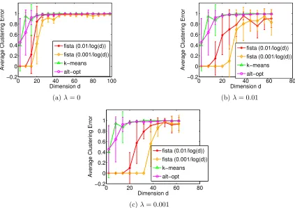
method becomes more robust to noisy dimensions. As observed earlier, the performance of FISTA is also sensitive to the choice ofε.
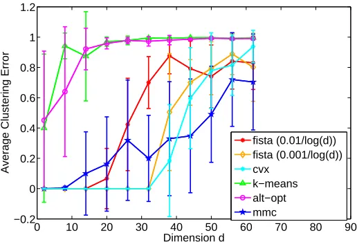
Finally we give a comparison of sparse discriminative clustering (cvx and FISTA) with max-margin clustering (Li et al., 2009) in Figure 5. We note that square loss is used in our framework whereas hinge loss is used in max-margin clustering. We have also included the behavior of K-means and alternating optimization methods in Figure 5 for completeness. From this plot, it is clear that the max-margin clustering is sensitive to noisy dimensions present in the data. Sparse discriminative clustering with square loss is able to maintain zero cluster error for a large number of noisy dimensions, while the performance of max-margin clustering starts deteriorating after adding a few noisy dimensions. However, we note from Figure 5 that for large dimensions, the hinge loss used in max-margin clustering is observed to provide a better solution than the square loss used in our framework.
0 20 40 60 80 100
−0.2 0 0.2 0.4 0.6 0.8 1
Dimension d
Average Clustering Error
fista (0.01/log(d)) fista (0.001/log(d)) k−means alt−opt
(a)λ= 0
0 20 40 60 80
−0.2 0 0.2 0.4 0.6 0.8 1
Dimension d
Average Clustering Error
fista (0.01/log(d)) fista (0.001/log(d)) k−means alt−opt
(b)λ= 0.01
0 20 40 60 80
−0.2 0 0.2 0.4 0.6 0.8 1
Dimension d
Average Clustering Error
fista (0.01/log(d)) fista (0.001/log(d)) k−means alt−opt
(c)λ= 0.001
Figure 4: Comparison withk-means and alternating optimization,n= 100.
7.2 Experiments on real-world data
Experiments on two-class data. Experiments were conducted on real two-class clas-sification datasets2 to compare the performance of sparse discriminative clustering against non-sparse discriminative clustering, alternating optimization, K-means and max-margin
0 10 20 30 40 50 60 70 80 90 −0.2
0 0.2 0.4 0.6 0.8 1 1.2
Dimension d
Average Clustering Error
fista (0.01/log(d)) fista (0.001/log(d)) cvx
k−means alt−opt mmc
Figure 5: Comparison with k-means, alternating optimization and max-margin clustering (mmc), n = 100. The plots for FISTA, cvx and mmc correspond to the best choice of regularization parameters.
clustering algorithms. For sparse and non-sparse discriminative clustering, we consider the problem in Eq. (24) and the algorithm detailed in Section 6.3 (with the regularizationc= 0 for the non-sparse case). The alternating optimization method is described in Proposition 1. For the two-class datasets, the clustering performance for a cluster ¯y∈ {+1,−1}nobtained
from an algorithm under comparison, was computed as 1−(¯y>y/n)2, whereyis the original labeling. Here we explicitly compare the output of clustering with the original labels of the data points.
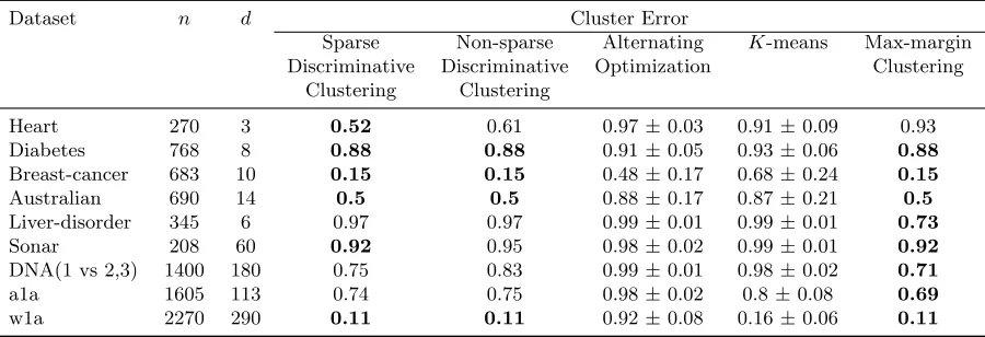
The dataset details and clustering performance results are summarized in Table 1. The experiments for discriminative clustering were conducted for different values of a, c∈ {10−3,10−2,10−1}1d associated with the`2-regularizer and`1-regularizer respectively. The range of cluster imbalance parameter was chosen to be ν ∈ {0.01,0.25,0.5,0.75,1}. Note that for ν 6= 1, the reformulation given in Eq. (14) was used, as explained after Eq. (17) in Section 3. The results given in Table 1 pertain to the best choices of these parame-ters. Similarly, the values of regularization parameter for max-margin clustering (Li et al., 2009) were chosen from the set {10−5,10−4,10−3,10−2,0.1,1,10} and the cluster balance parameter was chosen from{0.1,0.2, . . . ,0.9}. The results for alternating optimization and
significantly better than the non-sparse version with the hinge loss (see additional experi-ments in Figure 5). The results also show that adding sparse regularizers to discriminative clustering helps in a better cluster identification when compared to the non-sparse case.
Table 1: Experiments on two-class datasets
Dataset n d Cluster Error
Sparse Non-sparse Alternating K-means Max-margin
Discriminative Discriminative Optimization Clustering Clustering Clustering
Heart 270 3 0.52 0.61 0.97±0.03 0.91±0.09 0.93
Diabetes 768 8 0.88 0.88 0.91±0.05 0.93±0.06 0.88
Breast-cancer 683 10 0.15 0.15 0.48±0.17 0.68±0.24 0.15
Australian 690 14 0.5 0.5 0.88±0.17 0.87±0.21 0.5
Liver-disorder 345 6 0.97 0.97 0.99±0.01 0.99±0.01 0.73
Sonar 208 60 0.92 0.95 0.98±0.02 0.99±0.01 0.92
DNA(1 vs 2,3) 1400 180 0.75 0.83 0.99±0.01 0.98±0.02 0.71
a1a 1605 113 0.74 0.75 0.98±0.02 0.8±0.08 0.69
w1a 2270 290 0.11 0.11 0.92±0.08 0.16±0.06 0.11
Experiments on real multi-label data. Experiments were also conducted on the Mi-crosoft COCO dataset3 to demonstrate the effectiveness of the proposed method in discov-ering multiple labels. We consideredn= 2000 images from the dataset, each of which was labeled with a subset of K= 80 labels. The labels identified the objects in the images like person, car, chair, table, etc. and the corresponding features for each image were extracted from the last layer of a conventional convolutional neural network (CNN). The CNN was originally trained over the imagenet data (Krizhevsky et al., 2012).
For each image in the dataset, we obtained d = 1000 features. We then performed discriminative clustering on the 2000×1000 data matrixX and obtained the label matrix
Y which was then subjected to the alternating optimization procedure (see Section 5.3). It is clearly unlikely to recover perfect labels; therefore we now describe a way of mea-suring the amount of information which is recovered. In order to extract meaningful cluster information from the result so-obtained, we computed the correlation matrix Yk>ΠnYtrue
whereYtrue is then×K label matrix containing actual labels and Πn is then×ncentering
matrixIn−n11n1>n. Thekpredicted labels for the examples are present in theYkmatrix of
sizen×k. In order to choose an appropriate value ofk, we plotted Tr(ΦYtrueΦYk) (shown in Figure 6 along with aK-means baseline), where ΦYk =Yk(Yk
>Y
k)−1Yk>. From these plots,
we chosek= 30 to be a suitable value for our interpretation purposes.
After choosing an arbitrary value of k = 30, we plotted the correlations between the actual and predicted labels. The heat map of the normalized absolute correlations is given in Figure 7, where the columns and rows corresponding to the 80 true labels and 30 predicted labels respectively, are ordered according to the sum of squared correlations (the top-scoring labels appear to the left-bottom). From this plot, we extract following highly correlated
0 10 20 30 40 50 60 70 80 0
2 4 6 8 10 12
Num labels
T
r(
Φ
(
Yt
r
u
e
)
*
Φ
(
Yk
))
alt−min k−means
Figure 6: Plot of Tr(ΦYtrueΦYk).
True labels
Predicted labels
0.02 0.04 0.06 0.08 0.1 0.12
Figure 7: Heat map of correlations,Yk>ΠnYtruewithk= 30, with columns and rows ordered
according to the sum of squared correlations.
labels: person, dining table, car, chair, cup, tennis racket, bowl, truck, fork, pizza, showing that these labels were partially recovered by our unsupervised technique (note that the CNN features are learned with supervision on the different dataset Imagenet, hence there is still some partial supervision).
8. Conclusion
analysis to l-sparse case with higher l, extending the framework to nonlinear clustering using kernels, considering related weakly supervised learning extensions (Joulin and Bach, 2012), going beyond uniqueness of rank-one solutions, and improving the complexity of our algorithm to O(nd), for example using stochastic gradient techniques.
Acknowledgments
References
Jean-Baptiste Alayrac, Piotr Bojanowski, Nishant Agrawal, Ivan Laptev, Josef Sivic, and Simon Lacoste-Julien. Unsupervised learning from narrated instruction videos. In Com-puter Vision and Pattern Recognition (CVPR), 2016.
D. Arthur and S. Vassilvitskii. k-means++: The advantages of careful seeding. In Proceed-ings of the eighteenth annual ACM-SIAM symposium on Discrete algorithms, 2007.
F. Bach and Z. Harchaoui. DIFFRAC : a discriminative and flexible framework for cluster-ing. InAdvances in Advances in Neural Information Processing Systems (NIPS), 2007.
F. Bach, R. Jenatton, J. Mairal, and G. Obozinski. Optimization with sparsity-inducing penalties. Foundations and TrendsR in Machine Learning, 4(1):1–106, 2012.
A. Beck and M. Teboulle. A fast iterative shrinkage-thresholding algorithm for linear inverse problems. SIAM J. Imaging Sci., 2(1):183–202, 2009.
R. Bellman. A note on cluster analysis and dynamic programming. Mathematical Bio-sciences, 1973.
G. Blanchard, M. Kawanabe, M. Sugiyama, V. Spokoiny, and K.-R. M¨uller. In search of non-Gaussian components of a high-dimensional distribution. The Journal of Machine Learning Research, 7:247–282, 2006.
Piotr Bojanowski, Francis Bach, Ivan Laptev, Jean Ponce, Cordelia Schmid, and Josef Sivic. Finding actors and actions in movies. In Proc. IEEE International Conference on Computer Vision, 2013.
J. M. Borwein and A. S. Lewis. Convex Analysis and Nonlinear Optimization, volume 3 of CMS Books in Mathematics/Ouvrages de Math´ematiques de la SMC. Springer-Verlag, 2000. Theory and examples.
N. Boumal, B. Mishra, P.-A. Absil, and R. Sepulchre. Manopt, a Matlab Toolbox for Optimization on Manifolds. Journal of Machine Learning Research, 2014.
J. Bourgain, V. H. Vu, and P. M. Wood. On the singularity probability of discrete random matrices. Journal of Functional Analysis, 258(2):559–603, 2010.
S. Boyd and L. Vandenberghe. Convex optimization. Cambridge University Press, Cam-bridge, 2004.
T. De Bie and N. Cristianini. Convex methods for transduction. In Advances in Neural Information Processing Systems (NIPS), pages 73–80, 2003.
F. De la Torre and T. Kanade. Discriminative cluster analysis. In Proceedings of the conference on machine learning (ICML), 2006.
C. Ding and T. Li. Adaptive dimension reduction using discriminant analysis and K-means clustering. In Proceedings of the conference on machine learning (ICML), 2007.
D. Freedman. Statistical models: theory and practice. Cambridge University Press, 2009.
J. H. Friedman and W. Stuetzle. Projection pursuit regression. Journal of the American statistical Association, 76(376):817–823, 1981.
A. Frieze and M. Jerrum. Improved approximation algorithms for MAX k-CUT and MAX BISECTION. In Integer Programming and Combinatorial Optimization. Springer, 1995.
M. R. Garey, D. S. Johnson, and L. Stockmeyer. Some simplified NP-complete graph problems. Theoret. Comput. Sci., 1(3):237–267, 1976.
M. X. Goemans and D. P. Williamson. Improved Approximation Algorithms for Maximum Cut and Satisfiability Problems Using Semidefinite Programming. J. ACM, 42(6):1115– 1145, November 1995.
J. C. Gower and G. J. S. Ross. Minimum spanning trees and single Linkage cluster analysis. Journal of the Royal Statistical Society. Series C (Applied Statistics), 18(1), 1969.
M. Grant and S. Boyd. Graph implementations for nonsmooth convex programs. In V. Blon-del, S. Boyd, and H. Kimura, editors,Recent Advances in Learning and Control, Lecture Notes in Control and Information Sciences, pages 95–110. Springer-Verlag Limited, 2008.
M. Grant and S. Boyd. CVX: Matlab Software for Disciplined Convex Programming, version 2.1, March 2014.
Edouard Grave. A convex relaxation for weakly supervised relation extraction. InEMNLP, 2014.
G. Huang, J. Zhang, S. Song, and Z. Chen. Maximin separation probability clustering. In Proceedings of the AAAI Conference on Artificial Intelligence, 2015.
A. Hyv¨arinen, J. Karhunen, and E. Oja. Independent component analysis, volume 46. John Wiley & Sons, 2004.
A. Joulin and F. Bach. A convex relaxation for weakly supervised classifiers. InProceedings of the conference on machine learning (ICML), 2012.
A. Joulin, F. Bach, and J. Ponce. Discriminative clustering for image co-segmentation. In Proc. CVPR, 2010a.
A. Joulin, J. Ponce, and F. Bach. Efficient optimization for discriminative latent class models. In Advances in Advances in Neural Information Processing Systems (NIPS), 2010b.
A. T. Kalai, A. Moitra, and G. Valiant. Efficiently learning mixtures of two Gaussians. In International Symposium on Theory of Computing (STOC), pages 553–562, 2010.
R. M. Karp. Reducibility among combinatorial problems. In Complexity of computer computations, pages 85–103. Plenum, New York, 1972.
A. Krizhevsky, I. Sutskever, and G. E. Hinton. ImageNet Classification with Deep Con-volutional Neural Networks. In Advances in Advances in Neural Information Processing Systems (NIPS), 2012.
R´emi Lajugie, Piotr Bojanowski, Philippe Cuvillier, Sylvain Arlot, and Francis Bach. A weakly-supervised discriminative model for audio-to-score alignment. In Proc. IEEE International Conference on Acoustics, Speech, and Signal Processing, 2016.
N. Le Roux and F. Bach. Local component analysis. In Proceedings of the International Conference on Learning Representations, 2013.
Y.-F. Li, I. W. Tsang, J. T.-Y. Kwok, and Z-H. Zhou. Tighter and convex maximum margin clustering. In AISTATS, pages 344–351, 2009.
Z. Q. Luo, W. K. Ma, A. C. So, Y. Ye, and S. Zhang. Semidefinite relaxation of quadratic optimization problems. Signal Processing Magazine, IEEE, 2010.
J. B. MacQueen. Some Methods for Classification and Analysis of MultiVariate Observa-tions. InProc. of the fifth Berkeley Symposium on Mathematical Statistics and Probability, volume 1, pages 281–297. University of California Press, 1967.
A. Moitra and G. Valiant. Settling the polynomial learnability of mixtures of Gaussians. In Annual Symposium on Foundations of Computer Science (FOCS), pages 93–102, 2010.
Y. Nesterov. Smoothing technique and its applications in semidefinite optimization. Math. Program., 2007.
A. Y. Ng, M. I. Jordan, and Y. Weiss. On Spectral Clustering: Analysis and an algorithm. In T.G. Dietterich, S. Becker, and Z. Ghahramani, editors, Advances in Advances in Neural Information Processing Systems (NIPS). 2002.
G. Niu, B. Dai, L. Shang, and M. Sugiyama. Maximum volume clustering: a new discrim-inative clustering approach. Journal of Machine Learning Research, 14(1):2641–2687, 2013.
R. Ostrovsky, Y. Rabani, L. J. Schulman, and C. Swamy. The effectiveness of lloyd-type methods for the k-means problem. In Annual Symposium on Foundations of Computer Science (FOCS), pages 165–176, 2006.
P. H Sch¨onemann. A generalized solution of the orthogonal Procrustes problem. Psychome-trika, 31(1), 1966.
J. Tropp. User-friendly tail bounds for sums of random matrices. Found. Comput. Math., 2012.
J. von Neumann. Thermodynamik quantummechanischer Gesamheiten. G¨ott. Nach, (1): 273–291, 1927.
F. Wang, B. Zhao, and C. Zhang. Linear time maximum margin clustering. IEEE Trans-actions on Neural Networks, 2010.
H. Wang, F. Nie, and H. Huang. Multi-View Clustering and Feature Learning via Structured Sparsity. InProceedings of the conference on machine learning (ICML), volume 28, 2013.
Z. Wen, D. Goldfarb, and K. Scheinberg. Block coordinate descent methods for semidef-inite programming. In Handbook on Semidefinite, Conic and Polynomial Optimization. Springer, 2012.
L. Xu, J. Neufeld, B. Larson, and D. Schuurmans. Maximum margin clustering. InAdvances in Advances in Neural Information Processing Systems (NIPS), 2004.
J. Ye, Z. Zhao, and M. Wu. Discriminative k-means for clustering. InAdvances in Advances in Neural Information Processing Systems (NIPS), 2008.
Appendix A. Joint clustering and dimension reduction
Given y, we need to optimize the Rayleigh quotient w>wX>>Xyy>Xw>Xw with a rank-one matrix
in the numerator, which leads to w = (X>X)−1X>y. Given w, we will show that the averaged distortion measure of K-means once the means have been optimized is exactly equal to (y>ΠnXw)2/kΠnyk22. Given the data matrix X ∈Rn×d, K-means to cluster the data into two components will tend to approximate the data points in X by the centroids
c+∈Rdand c−∈Rdsuch that
X ≈ (y+ 1n)
2 c
>
+−
(y−1n)
2 c
>
− (since y∈ {−1,1}n)
= y 2(c
>
+−c>−) +
1 21n(c
>
++c>−).
The objective of K-means can now be written as problemKM:
min
y,c+,c−
X−y
2(c
>
+−c>−)−
1 21n(c
>
++c>−)
2 F = min
y,c+,c−
X− (y+ 1n)
2 c
>
+−
(1n−y)
2 c > − 2 F = min
y,c+,c−
kXk2
F +kc>+k2F
(y+ 1n)
2 2
+kc>−k2 F
(1−yn)
2 2
+ 2c>−c+
(y+ 1n)
2
>
(1n−y)
2
−2 trX>
(y+ 1n)
2 c
>
++
(1n−y)
2 c
> −
= min
y,c+,c−
kXk2F +kc>+k2F1
2(n+ 1
>
ny) +kc > −k2F
1 2(n−1
>
ny)−2c >
+X
>
y+ 1n
2
−2c>−X>
1n−y
2
.
Fixingy and minimizing with respect to c+ and c−, we get closed-form expressions forc+ and c− as
c+=
X>(y+ 1n)
(n+ 1> ny)
and c− =
X>(1n−y)
(n−1> ny)